
Download Lectures on Biostatistics (1971). Corrected and searchable version of Google books edition
Download review of Lectures on Biostatistics (THES, 1973).
This post is now a bit out of date: there is a summary of my more recent efforts (papers, videos and pop stuff) can be found on Prof Sivilotti’s OneMol pages.
What follows is a simplified version of part of a paper that appeared as a preprint on arXiv in July. It appeared as a peer-reviewed paper on 19th November 2014, in the new Royal Society Open Science journal. If you find anything wrong, or obscure, please email me. Be vicious.
There is also a simplified version, given as a talk on Youtube..
It’s a follow-up to my very first paper, which was written in 1959 – 60, while I was a fourth year undergraduate(the history is at a recent blog). I hope this one is better.
‘”. . . before anything was known of Lydgate’s skill, the judgements on it had naturally been divided, depending on a sense of likelihood, situated perhaps in the pit of the stomach, or in the pineal gland, and differing in its verdicts, but not less valuable as a guide in the total deficit of evidence” ‘George Eliot (Middlemarch, Chap. 45)
“The standard approach in teaching, of stressing the formal definition of a p-value while warning against its misinterpretation, has simply been an abysmal failure” Sellke et al. (2001) `The American Statistician’ (55), 62–71
The last post was about screening. It showed that most screening tests are useless, in the sense that a large proportion of people who test positive do not have the condition. This proportion can be called the false discovery rate. You think you’ve discovered the condition, but you were wrong.
Very similar ideas can be applied to tests of significance. If you read almost any scientific paper you’ll find statements like “this result was statistically significant (P = 0.047)”. Tests of significance were designed to prevent you from making a fool of yourself by claiming to have discovered something, when in fact all you are seeing is the effect of random chance. In this case we define the false discovery rate as the probability that, when a test comes out as ‘statistically significant’, there is actually no real effect.
You can also make a fool of yourself by failing to detect a real effect, but this is less harmful to your reputation.
It’s very common for people to claim that an effect is real, not just chance, whenever the test produces a P value of less than 0.05, and when asked, it’s common for people to think that this procedure gives them a chance of 1 in 20 of making a fool of themselves. Leaving aside that this seems rather too often to make a fool of yourself, this interpretation is simply wrong.
The purpose of this post is to justify the following proposition.
|
If you observe a P value close to 0.05, your false discovery rate will not be 5%. It will be at least 30% and it could easily be 80% for small studies.
|
This makes slightly less startling the assertion in John Ioannidis’ (2005) article, Why Most Published Research Findings Are False. That paper caused quite a stir. It’s a serious allegation. In fairness, the title was a bit misleading. Ioannidis wasn’t talking about all science. But it has become apparent that an alarming number of published works in some fields can’t be reproduced by others. The worst offenders seem to be clinical trials, experimental psychology and neuroscience, some parts of cancer research and some attempts to associate genes with disease (genome-wide association studies). Of course the self-correcting nature of science means that the false discoveries get revealed as such in the end, but it would obviously be a lot better if false results weren’t published in the first place.
How can tests of significance be so misleading?
Tests of statistical significance have been around for well over 100 years now. One of the most widely used is Student’s t test. It was published in 1908. ‘Student’ was the pseudonym for William Sealy Gosset, who worked at the Guinness brewery in Dublin. He visited Karl Pearson’s statistics department at UCL because he wanted statistical methods that were valid for testing small samples. The example that he used in his paper was based on data from Arthur Cushny, the first holder of the chair of pharmacology at UCL (subsequently named the A.J. Clark chair, after its second holder)
The outcome of a significance test is a probability, referred to as a P value. First, let’s be clear what the P value means. It will be simpler to do that in the context of a particular example. Suppose we wish to know whether treatment A is better (or worse) than treatment B (A might be a new drug, and B a placebo). We’d take a group of people and allocate each person to take either A or B and the choice would be random. Each person would have an equal chance of getting A or B. We’d observe the responses and then take the average (mean) response for those who had received A and the average for those who had received B. If the treatment (A) was no better than placebo (B), the difference between means should be zero on average. But the variability of the responses means that the observed difference will never be exactly zero. So how big does it have to be before you discount the possibility that random chance is all you were seeing. You do the test and get a P value. Given the ubiquity of P values in scientific papers, it’s surprisingly rare for people to be able to give an accurate definition. Here it is.
|
The P value is the probability that you would find a difference as big as that observed, or a still bigger value, if in fact A and B were identical.
|
If this probability is low enough, the conclusion would be that it’s unlikely that the observed difference (or a still bigger one) would have occurred if A and B were identical, so we conclude that they are not identical, i.e. that there is a genuine difference between treatment and placebo.
This is the classical way to avoid making a fool of yourself by claiming to have made a discovery when you haven’t. It was developed and popularised by the greatest statistician of the 20th century, Ronald Fisher, during the 1920s and 1930s. It does exactly what it says on the tin. It sounds entirely plausible.
What could possibly go wrong?
Another way to look at significance tests
One way to look at the problem is to notice that the classical approach considers only what would happen if there were no real effect or, as a statistician would put it, what would happen if the null hypothesis were true. But there isn’t much point in knowing that an event is unlikely when the null hypothesis is true unless you know how likely it is when there is a real effect.
We can look at the problem a bit more realistically by means of a tree diagram, very like that used to analyse screening tests, in the previous post.
In order to do this, we need to specify a couple more things.
First we need to specify the power of the significance test. This is the probability that we’ll detect a difference when there really is one. By ‘detect a difference’ we mean that the test comes out with P < 0.05 (or whatever level we set). So it’s analogous with the sensitivity of a screening test. In order to calculate sample sizes, it’s common to set the power to 0.8 (obviously 0.99 would be better, but that would often require impracticably large samples).
The second thing that we need to specify is a bit trickier, the proportion of tests that we do in which there is a real difference. This is analogous to the prevalence of the disease in the population being tested in the screening example. There is nothing mysterious about it. It’s an ordinary probability that can be thought of as a long-term frequency. But it is a probability that’s much harder to get a value for than the prevalence of a disease.
If we were testing a series of 30C homeopathic pills, all of the pills, regardless of what it says on the label, would be identical with the placebo controls so the prevalence of genuine effects, call it P(real), would be zero. So every positive test would be a false positive: the false discovery rate would be 100%. But in real science we want to predict the false discovery rate in less extreme cases.
Suppose, for example, that we test a large number of candidate drugs. Life being what it is, most of them will be inactive, but some will have a genuine effect. In this example we’d be lucky if 10% had a real effect, i.e. were really more effective than the inactive controls. So in this case we’d set the prevalence to P(real) = 0.1.
We can now construct a tree diagram exactly as we did for screening tests.
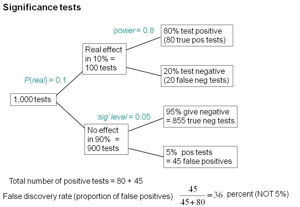
Suppose that we do 1000 tests. In 90% of them (900 tests) there is no real effect: the null hypothesis is true. If we use P = 0.05 as a criterion for significance then, according to the classical theory, 5% of them (45 tests) will give false positives, as shown in the lower limb of the tree diagram. If the power of the test was 0.8 then we’ll detect 80% of the real differences so there will be 80 correct positive tests.
The total number of positive tests is 45 + 80 = 125, and the proportion of these that are false positives is 45/125 = 36 percent. Our false discovery rate is far bigger than the 5% that many people still believe they are attaining.
In contrast, 98% of negative tests are right (though this is less surprising because 90% of experiments really have no effect).
The equation
You can skip this section without losing much.
As in the case of screening tests, this result can be calculated from an equation. The same equation works if we substitute power for sensitivity, P(real) for prevalence, and siglev for (1 – specificity) where siglev is the cut off value for “significance”, 0.05 in our examples.
The false discovery rate (the probability that, if a “signifcant” result is found, there is actually no real effect) is given by
\[FDR = \frac{siglev\left(1-P(real)\right)}{power.P(real) + siglev\left(1-P(real)\right) }\; \]
In the example above, power = 0.8, siglev = 0.05 and P(real) = 0.1, so the false discovery rate is
\[\frac{0.05 (1-0.1)}{0.8 \times 0.1 + 0.05 (1-0.1) }\; = 0.36 \]
So 36% of “significant” results are wrong, as found in the tree diagram.
Some subtleties
The argument just presented should be quite enough to convince you that significance testing, as commonly practised, will lead to disastrous numbers of false positives. But the basis of how to make inferences is still a matter that’s the subject of intense controversy among statisticians, so what is an experimenter to do?
It is difficult to give a consensus of informed opinion because, although there is much informed opinion, there is rather little consensus. A personal view follows. Colquhoun (1970), Lectures on Biostatistics, pp 94-95.
This is almost as true now as it was when I wrote it in the late 1960s, but there are some areas of broad agreement.
There are two subtleties that cause the approach outlined above to be a bit contentious. The first lies in the problem of deciding the prevalence, P(real). You may have noticed that if the frequency of real effects were 50% rather than 10%, the approach shown in the diagram would give a false discovery rate of only 6%, little different from the 5% that’s embedded in the consciousness of most experimentalists.
But this doesn’t get us off the hook, for two reasons. For a start, there is no reason at all to think that there will be a real effect there in half of the tests that we do. Of course if P(real) were even bigger than 0.5, the false discovery rate would fall to zero, because when P(real) = 1, all effects are real and therefore all positive tests are correct.
There is also a more subtle point. If we are trying to interpret the result of a single test that comes out with a P value of, say, P = 0.047, then we should not be looking at all significant results (those with P < 0.05), but only at those tests that come out with P = 0.047. This can be done quite easily by simulating a long series of t tests, and then restricting attention to those that come out with P values between, say, 0.045 and 0.05. When this is done we find that the false discovery rate is at least 26%. That’s for the best possible case where the sample size is good (power of the test is 0.8) and the prevalence of real effects is 0.5. When, as in the tree diagram, the prevalence of real effects is 0.1, the false discovery rate is 76%. That’s enough to justify Ioannidis’ statement that most published results are wrong.
One problem with all of the approaches mentioned above was the need to guess at the prevalence of real effects (that’s what a Bayesian would call the prior probability). James Berger and colleagues (Sellke et al., 2001) have proposed a way round this problem by looking at all possible prior distributions and so coming up with a minimum false discovery rate that holds universally. The conclusions are much the same as before. If you claim to have found an effects whenever you observe a P value just less than 0.05, you will come to the wrong conclusion in at least 29% of the tests that you do. If, on the other hand, you use P = 0.001, you’ll be wrong in only 1.8% of cases. Valen Johnson (2013) has reached similar conclusions by a related argument.
A three-sigma rule
As an alternative to insisting on P < 0.001 before claiming you’ve discovered something, you could use a 3-sigma rule. In other words, insist that an effect is at least three standard deviations away from the control value (as opposed to the two standard deviations that correspond to P = 0.05).
The three sigma rule means using P= 0.0027 as your cut off. This, according to Berger’s rule, implies a false discovery rate of (at least) 4.5%, not far from the value that many people mistakenly think is achieved by using P = 0.05 as a criterion.
Particle physicists go a lot further than this. They use a 5-sigma rule before announcing a new discovery. That corresponds to a P value of less than one in a million (0.57 x 10⁻⁶). According to Berger’s rule this corresponds to a false discovery rate of (at least) around 20 per million. Of course their experiments can’t be randomised usually, so it’s as well to be on the safe side.
Underpowered experiments
All of the problems discussed so far concern the near-ideal case. They assume that your sample size is big enough (power about 0.8 say) and that all of the assumptions made in the test are true, that there is no bias or cheating and that no negative results are suppressed. The real-life problems can only be worse. One way in which it is often worse is that sample sizes are too small, so the statistical power of the tests is low.
The problem of underpowered experiments has been known since 1962, but it has been ignored. Recently it has come back into prominence, thanks in large part to John Ioannidis and the crisis of reproducibility in some areas of science. Button et al. (2013) said
“We optimistically estimate the median statistical power of studies in the neuroscience field to be between about 8% and about 31%”
This is disastrously low. Running simulated t tests shows that with a power of 0.2, not only do you have only a 20% chance of detecting a real effect, but that when you do manage to get a “significant” result there is a 76% chance that it’s a false discovery.
And furthermore, when you do find a “significant” result, the size of the effect will be over-estimated by a factor of nearly 2. This “inflation effect” happens because only those experiments that happen, by chance, to have a larger-than-average effect size will be deemed to be “significant”.
What should you do to prevent making a fool of yourself?
The simulated t test results, and some other subtleties, will be described in a paper, and/or in a future post. But I hope that enough has been said here to convince you that there are real problems in the sort of statistical tests that are universal in the literature.
The blame for the crisis in reproducibility has several sources.
One of them is the self-imposed publish-or-perish culture, which values quantity over quality, and which has done enormous harm to science.
The mis-assessment of individuals by silly bibliometric methods has contributed to this harm. Of all the proposed methods, altmetrics is demonstrably the most idiotic. Yet some vice-chancellors have failed to understand that.
Another is scientists’ own vanity, which leads to the PR department issuing disgracefully hyped up press releases.
In some cases, the abstract of a paper states that a discovery has been made when the data say the opposite. This sort of spin is common in the quack world. Yet referees and editors get taken in by the ruse (e.g see this study of acupuncture).
The reluctance of many journals (and many authors) to publish negative results biases the whole literature in favour of positive results. This is so disastrous in clinical work that a pressure group has been started; altrials.net “All Trials Registered | All Results Reported”.
Yet another problem is that it has become very hard to get grants without putting your name on publications to which you have made little contribution. This leads to exploitation of young scientists by older ones (who fail to set a good example). Peter Lawrence has set out the problems.
And, most pertinent to this post, a widespread failure to understand properly what a significance test means must contribute to the problem. Young scientists are under such intense pressure to publish, they have no time to learn about statistics.
Here are some things that can be done.
- Notice that all statistical tests of significance assume that the treatments have been allocated at random. This means that application of significance tests to observational data, e.g. epidemiological surveys of diet and health, is not valid. You can’t expect to get the right answer. The easiest way to understand this assumption is to think about randomisation tests (which should have replaced t tests decades ago, but which are still rare). There is a simple introduction in Lectures on Biostatistics (chapters 8 and 9). There are other assumptions too, about the distribution of observations, independence of measurements), but randomisation is the most important.
- Never, ever, use the word “significant” in a paper. It is arbitrary, and, as we have seen, deeply misleading. Still less should you use “almost significant”, “tendency to significant” or any of the hundreds of similar circumlocutions listed by Matthew Hankins on his Still not Significant blog.
- If you do a significance test, just state the P value and give the effect size and confidence intervals (but be aware that this is just another way of expressing the P value approach: it tells you nothing whatsoever about the false discovery rate).
- Observation of a P value close to 0.05 means nothing more than ‘worth another look’. In practice, one’s attitude will depend on weighing the losses that ensue if you miss a real effect against the loss to your reputation if you claim falsely to have made a discovery.
- If you want to avoid making a fool of yourself most of the time, don’t regard anything bigger than P < 0.001 as a demonstration that you’ve discovered something. Or, slightly less stringently, use a three-sigma rule.
Despite the gigantic contributions that Ronald Fisher made to statistics, his work has been widely misinterpreted. We must, however reluctantly, concede that there is some truth in the comment made by an astute journalist:
“The plain fact is that 70 years ago Ronald Fisher gave scientists a mathematical machine for turning baloney into breakthroughs, and °flukes into funding. It is time to pull the plug“. Robert Matthews Sunday Telegraph, 13 September 1998.
There is now a video on YouTube that attempts to explain explain simply the essential ideas. The video has now been updated. The new version has better volume and it used term ‘false positive risk’, rather than the earlier term ‘false discovery rate’, to avoid confusion with the use of the latter term in the context of multiple comparisons.
The false positive risk: a proposal concerning what to do about p-values (version 2)
Follow-up
31 March 2014 I liked Stephen Senn’s first comment on twitter (the twitter stream is storified here). He said ” I may have to write a paper ‘You may believe you are NOT a Bayesian but you’re wrong'”. I maintain that the analysis here is merely an exercise in conditional probabilities. It bears a formal similarity to a Bayesian argument, but is free of more contentious parts of the Bayesian approach. This is amplified in a comment, below.
4 April 2014
I just noticed that my first boss, Heinz Otto Schild.in his 1942 paper about the statistical analysis of 2+2 dose biological assays (written while he was interned at the beginning of the war) chose to use 99% confidence limits, rather than the now universal 95% limits. The later are more flattering to your results, but Schild was more concerned with precision than self-promotion.

*If you know what you are doing, your false discovery rate is 100%. Anything less is an improvement. You may be learning something.
*on screening: using significance tests for industrial/science screen is doing it wrong. Look at ranking and selection procedures.
@billraynor
Thanks for your comment, but I’m afraid that I don’t understand your points at all, especially the first one.
* When your hypothesis is correct, then any “significant” result is a false positive. If you think singificance is a “discovery”, then your FDR is 100%. So an 80% false discovery rate is an improvement over that. Fisher was real clear about the need for replication. A significant result only says at least one of your sub-hypotheses could be wrong, not which one. (e.g. normality and/or heteroscedasticity could fail when the means are equal).
*The second comment is on the misuse of significance testing for screening. Using plain old significance testing for screening is basically “asking for it”. If your real objective is screening, there are statistical procedures designed specifically for that, generally referred to as “ranking and selection” procedures, introduced by Bechhofer in the 1950’s. As always, these things are intertwined, so I can make an FDR output match a subset selction output, but the subset selection methods are clearer on their objectives and avoid the whole “significance” semantic confusion.
*It is instructive to go back to the paper by Student that DC cites and anybody doing so will be puzzled by a huge numerical discrepancy. Student used the Cushny & Peebles data to illustrate his “Bayesian” approach (“Bayesian” in inverted commas because although the technique was ubiquitous the term was not) and so did Fisher. In fact they both got the numbers wrong (Student copied them incorrectly and Fisher copied Student). However, the numerical discrepancy in probabilities is not between Student and Fisher but between both of them & the alternative Bayesian approach DC presents here. (I know that DC doesn’t like being labelled Bayesian but that is what you have here.)
Statisticians like Student & Pearson regularly used inverse probability arguments. They used Laplace’s device of an uninformative prior distribution and if you do that you can interpret one-sided P-values in terms of posterior probabilities. Fisher didn’t like this, having read the critical arguments of Venn and others on Lapace’s principle of insufficent reason, and he gave an alternative explanation of a probability as extreme or more extreme than the value observed if the null hypothesis were true. Actually, you can also find this interpretation in the “Bayesian” Karl Pearson, although he usually favoured the Bayesian interpretation.
It was Harold Jeffreys who, much impressed by Broad’s argument against attempting to prove scientific laws using the then standard “Bayesian” machinery. Broad had shown that with an uninformative prior you could never prove a scientifc law was even probable, since the number of potential future instances would always outweigh those that had been seen. (The difference between predicting the next observation and all future observations often confuses amateurs attempting to use Bayes theorem.) Jeffreys proposed that this could be addressed by having a lump of probability that the precise null was true. It the significance test that he developed to address this that gives radically different numbers to P-values.
Thus you should know that it very much depends what you believe regarding the null hypothesis (is a precise or a dividing hypothesis, to use David Cox’s distinction) and also regarding the alternative hypothesis as to what you will come up with. In fact it is possible to design examples in which two Bayesians will have the same prior probability that the alternative hypothesis is true and the same conditional probability for the true effect if the alternative hypothesis is true but, having seen exactly the same data will have posterior probabilities that differ strongly: one now believeing in the null and the other in the alternative.
However, provided you accept that significance tests are what they are and don’t try to make them something else, (if you want to be Bayesian, for goodness sake, be Bayesian) then they do have a limited use. You need to stop being worried about making a fool of yourself. That will happen all the time. In fact you can’t avoid it. If you demand much more stringent significance levels and you take the (in my view admirable) attitude that you certainly should publish negative results, then you run the risk of making a fool of yourself by claiming there is no effect unless you design much bigger experiments. However, in many scientific disciplines designing huge experiments doesn’t make sense.
I think it is sensible to regard the conventional 5% level as suggesting, as David implies, ‘worth a second look’. However, I also think it is a mistake to regard recalibrated P-values as being a sensible approach to anything. If you want inverse probabilities, calculate them.
(See http://arxiv.org/pdf/1001.2975.pdf for a discussion of Jeffreys and Broad)
@Stephen Senn
Thanks very much for taking the time to respond. Of course I agree that negative results should be published.
Your paper, “Two Cheers for P values” should perhaps be read by anyone interested in the controversies.
As an outsider, I’ve been intrigued most of my life by the internecine strife between professional statisticians about the most fundamental aspects of their subject. As I said,
As you probably noticed, I assiduously avoided using the word “Bayesian”, in the vain hope of avoiding some of the controversy. The conclusions from the tree diagram come from nothing but counting, and they seem to me to be incontestable.
Hi David, very nice article. Three points (I hope constructive) I’d like to make:
(1) You mention the difference between randomized & non-randomized experiments, but I feel this could be clarified. Each class of experiment has the same capability to recognize correlation, but the non-randomized can not (unless other variables are measured) diagnose the causal hierarchy. If correlation is all that is being claimed, then even with an observational study, you can expect to get the right answer, just as much (ceteris paribus) as with an RCT.
(2) You mention applying more stringent tests, e.g. 3 sigma or 5 sigma. This doesn’t seem to me to fix the problem. As long as any p-value is used as a metric for summarizing an experimental result, information (prior information) is being needlessly discarded. By simply making the test more stringent, one’s ability to detect a real effect is compromised. Why not just incorporate all the available information and deliver a posterior distribution?
I have criticized the analysis of the Higgs boson data (I know, very unsporting) for use of the 5 sigmas approach in a blog article, The Higgs Boson at 5 Sigmas
(3)If my second point were implemented, it seems to me that another major problem with interpreting p-values would be eliminated. Whenever somebody does an experiment, the aim is to learn something about the true state of the universe, something that would be described by P(H|D), yet what people are being encouraged to report is (approximately) P(D|H). The desire to have the former is so great that I think people just can’t help attaching that interpretation to the latter (the base rate fallacy), even after they have been taught not to. The allure is too overpowering. (Examples in the same article I linked to above seem to support this.)
@aggressivePerfector
(1) My comment about randomisation is based in part on the fact that randomisation (permutation) tests are uniformly most powerful. The can also be done with no maths at all. I can’t imagine why anybody uses a t test these days. Another merit is that they make quite explicit the assumption of randomisation. If you apply significance tests to non-randomised data, all you do is to add an air of verisimilitude to an otherwise bald an unconvincing narrative.
(2) I tried to cover this with “one’s attitude will depend on weighing the losses that ensue if you miss a real effect against the loss to your reputation if you claim falsely to have made a discovery.”
(3) You suggest that it would be best simply to show a posterior distribution. The problem with this procedure is that it requires assumptions about the prior distribution, so every Bayesian will potentially produce a different result. That’s why I tried, as far is it’s possible, to avoid methods that specify an explicit prior distribution. That seems to me to be one of the advantages of the Berger approach.
*The conclusion from the tree diagram does not come from counting anything except a hypothetical model (so one in your head). The conclusion, of course, is model dependent. Is the model reasonable? If you are actually going to count, then having data helps. Here’s an interesting paper on the subject http://www.nature.com/nature/journal/v500/n7463/full/500395a.html
If one is testing dividing as opposed to precise hypotheses, then the situation is rather different. hence the fact that Karl Pearson could calculate a probability and give it both a Bayesian and P-value interpretation. More generally, however, unless you expect a P-value to be a posterior probability, there’s no problem with P-values. Furthermore, since it has never been easier to calculate a posterior probability than now there seems to be no excuse for not doing so for those who are interested in them. However, as Fisher pointed out, a combination of very low P-values and moderate posterior probabilities is worrying – it may indicate that the assumptions as a whole are wrong.
@StephenSenn
The Nature reference you give is interesting, but it doesn’t seem to me to be relevant to the present discussion.
The only model that I can see in the tree diagram is the supposition that the person either has or has not got the condition. Many conditions show a more or less continuous spectrum of intensities so it become a bit arbitrary to define ill. But often it’s possible to set a reasonable threshold so there isn’t much approximation involved by saying that a person does, or does not, suffer from cancer or dementia.
Is there any other assumption that I’ve missed?
*The degree of belief in a hypothesis and the probability that particular data will arise given a hypothesis are of course different, but each crucially important, concepts. My own views about the misunderstandings that arise in science and law by confusing these concepts are set out elsewhere. I don’t see conventional significance tests as problematic, if one sticks to their proper interpretation. I don’t disagree with anything in DC’s article, but I think it perhaps worthwhile to keep things as simple as possible.
Tests measure how likely it is that a potentially interesting result (suggesting that a null hypothesis Ho isn’t true) would have arisen, to at least the same degree of interest, if Ho is true. This is what it says on the tin, and this is of course what it does, as expressed in DC’s 2nd box. As such, tests are useful and clear, and independent of one’s prior scientific beliefs. It is easy to understand that with multiple testing you will get roughly 1 in 20 of them coming out with P <0.05 even if you are looking for non-existent effects – hence the need to apply Bonferroni corrections and to replicate published results that have only modestly low P-values.
DC’s concern arises from the terminology often employed, that a low P-value enables you to ‘reject Ho’, albeit at a stated significance level. This sounds like a statement about belief in Ho, or what DC describes as a claim of ‘discovery’. Degrees of belief are certainly not encapsulated in P values. It is possible to use data in Bayesian ways to recalculate degrees of belief in hypotheses in the light of new data, given suitable priors. This is fine, but the result depends on one’s vision of other hypotheses that might explain the data and on one’s priors – it may be different for different scientists. A low P value doesn’t even mean one’s belief in the corresponding Ho should be lowered: the data may be less likely on the only plausible alternative hypotheses.
Should papers change significance testing criteria or require Bayesian arguments? Already they do ask for qualitative Bayesian argument, in the sense that a paper won’t be published if the Discussion doesn’t render the rejection or support of hypotheses plausible. I don’t think calculation of posterior probabilities, always based on uncertain priors, is the way to go. Reduced publication bias and seeing negative results play their proper part in science would be great. The most constructive thing would be for papers always to acknowledge what DC says: “Observation of a P value close to 0.05 means nothing more than ‘worth another look’.” If another look rejects the posited effect size with P<.05, it would take a stout heart (or a lot of money) to carry on.
@Tony Gardner-Medwin
Concerning your last remark, it’s worth noting that P values are not at all reproducible. Under the null hypothesis they have a uniform distribution. If you get P = 0.04 in one experiment, and repeat the same experiment, there’s at least a 50% chance that the replicate experiment will turn out “non-significant” (and a lot higher chance in under-powered experiments).
In the examples discussed here, the prior, the prevalence, is a perfectly concrete frequency, though it can’t be estimated as easily as in the screening example. But it is certainly reasonable to postulate that it’s a lot lower than 0.5 in the screening of drug candidates, and smaller still in genome association studies. That means there is a serious problem in interpretation of P, at least in that sort of study.
The virtue of the Berger approach is that it is independent of the details of the prior probability.
*The replication probabilities of P-values is a red-herring. It was raised by Steve Goodman and my answer was given in Statistic in Medicine here http://onlinelibrary.wiley.com/doi/10.1002/sim.1072/abstract . I showed that it is a property shared by Bayesian statements. See Deborah Mayo’s blog here http://errorstatistics.com/2012/05/10/excerpts-from-s-senns-letter-on-replication-p-values-and-evidence/ for a discussion
If you toss a coin once there is no chance at all that the proportion of heads will be 1/2. This does not make the probability statement meaningless.
@StephenSenn
I agree entirely that it’s a red herring, and say so in the full paper. I pointed it out merely because Tony Gardner-Medwin raised the matter.
Although it is entirely to be expected, it does, nonetheless, come as a bit of a shock to many non-statisticians. Did you see this video?
I’m not sure what brush I’m being tarred with here. I merely pointed out the obvious at the end of my comments. We all agree P=0.05 means you need to do more experiments, and helps you somewhat to believe this might be worthwhile. If there is no genuine effect and you repeat the experiment, there is a 79% chance that your enthusiasm will be dampened by an increased P-value when you combine the two results, and a 50% chance that your new data will ‘reject’ (at P<0.05) the hypothesis that the true effect size is equal to its MLE estimate from the first experiment (giving a combined P>0.16 for the 2 experiments). This says something about the value of experimental replication, not about the replicability of P-values.
New data is more likely to raise than lower a P-value if the null hypothesis is true. However, better than just using a P-value to characterise the result is of course to use P-values to calculate confidence limits (the range of hypotheses that would render the data quite likely – within a range that would include say 95% of replications), as argued in the video. In the illustration above, 95% confidence limits would extend from zero to twice the observed average in the first experiment, while after the second experiment (if it produced its most likely result under Ho), they would extend from -0.2 to +1.2 times the initial average.
@Tony Gardner-Medwin
The process of doing another experiment and combining the data gets you into a whole new set of problems, the problems of P hacking.
While I agree that it’s always a good idea to give the effect size and confidence intervals, that doesn’t solve the dilemma of false discovery rates.
Stephen Senn brought this up on twitter (it’s storified). He asked
To which I replied
It’s amazing to me that 250 years after Bayes’ paper, we are still arguing about these matters. They are amazingly subtle.
I’ve recently come across an interesting ‘real world’ (well, game world) example which incorporates many of the same issues (p values, or more generally significance testing, the rate of occurrence of ‘unusual’ events, and the issue of ‘false positives’). This is the problem of computer cheating in high-level chess, and detecting of the same.
Since the chess programmes now available for even hand-held devices are stronger (in a chess sense) than even elite-level players, the problem of players being potentially able to cheat using computer assistance is a major one. The most widely applicable way potentially to detect such cheating is retrospectively, by comparing human players’ choices of moves during the game to the choices made by the chess ‘engines’ (programmes) in the same game positions.
The question then becomes: how close a correspondence ‘proves’ cheating using a computer, absent any other physical evidence that a player has been cheating? And a related one, how often might a human player reach a high ‘match’ rate without actually having been cheating?
A discussion of this by computer science Prof Ken Regan from SUNY Buffalo, one of the people who has been using the ‘engine matching’ method, can be found here. From the question he poses at the end I get the impression he needs the input of some statistical colleagues.
You are too complacent about confidence intervals. 95% of confidence intervals may contain the true parameter but this is not the same as saying that 95% of confidence intervals that exclude zero do so correctly.
@Stephen Senn
I don’t think that I was being at all complacent. I said that confidence intervals don’t tell you about your false discovery rate. But I really like the way you put it it.
I feel uncomfortable in general about the practice of imposing cut-offs. Most phenomena are graded or numerical in terms of duration, severity, proportion or certainty and that imposing a cut-off point can obscure and distort the reasoning. I make this point in my latest response (#19) to your blog on screening tests. However, a similar principle applies to P values.
P values and confidence intervals relate to the means of a group of measurements or proportions. The ‘likelihoods’ in these cases may be probability densities. However, in the case of P values, the ‘likelihood’ represented by P is not about the result actually seen but about the result actually seen OR other more extreme hypothetical results that were NOT seen. The P value is thus the probability of one standardised hypothetical finding conditional on another standardised hypothetical finding. This provides a consistent index of reproducibility. Furthermore, when we calculate ‘power’ we base it on a hypothetical estimated finite ‘real’ value HR. But this finite value HR is not the complement of the finite value H0 (i.e. p(H0) ≠ 1- p(HR) and so we cannot apply Bayes rule to it which is:
p(H0/V) = [p(H0)*p(V/H0)] / [p(H0)*p(V/H0)+ [p(-0)*p(V/-0)]
when –0 is the complement of H0 so that p(-0) = 1 – p(H0).
I think therefore that a calculation of the ‘false discovery rate’ using Bayes rule cannot be applied to ‘P’ value outputs as ‘specificities’ and ‘power’ calculation outputs as ‘sensitivities’ unless I have misunderstood the reasoning.
However, I do agree with that a 5% P value or a 95% confidence interval that only just excludes a difference of zero does not suggest a high probability of replication (i.e. a low false discovery rate when repeated by others). This is because those repeat results of barely more than a zero difference would not be regarded as ‘replication’. So how similar should a result be to the original to ‘replicate’ it? The Bayesians may of course incorporate their own subjective priors. We would also study other factors (e.g. the soundness of the methods, clarity of the write-up and absence of hidden biases such as selective reporting of results where the less flattering studies are omitted) when estimating the probability of replication (i.e. the false discovery rate when readers repeat the study).
PS. In the above response, my character for ‘Not H0‘ was replaced by ‘-0‘ when it was uploaded to the site. Therefore for ‘-0‘. read ‘notH0‘.
You say
I don’t know why you say that. The examples that I give are based on simple counting, and I can’t see any part of them that’s contentious.
I carefully avoided using the term “Bayes” because that is associated with subjective probabilities and a great deal of argument.
I liked Stephen Senn’s first comment on twitter (the twitter stream is storified here). He said ” I may have to write a paper ‘You may believe you are NOT a Bayesian but you’re wrong’”. I maintain that the analysis here may bear a formal similarity to a Bayesian argument, but is free of more contentious parts of the Bayesian approach. The arguments that I have used contain no subjective probabilities, and are an application of obvious rules of conditional probabilities.
The classical example of Bayesian argument is the assessment of the evidence of the hypothesis that the earth goes round the sun. The probability of this hypothesis being true, given some data, must be subjective since it’s not possible to imagine a population of solar systems, some of which are heliocentric and some of which are not.
I argue that that problem of testing a series of drugs to see whether or not their effects differ from a control group is quite different. It’s easy to imagine a large number of candidate drugs some of which are active (fraction P(real) say) , some of which aren’t. So the prevalence (or prior, if you must) is a perfectly well-defined probability, which could be determined with sufficient effort. If you test one drug at random, the probability of it being active is P(real). It’s no different from the probability of picking a black ball from an urn that contains a fraction P(real) of black balls. to use the statisticians’ favourite example.
I agree that there is nothing contentious about your calculation, which is actually an un-contentious rearrangement of Bayes rule applied to a prevalence, sensitivity and false positive rate. Bayes rule is a simple piece of arithmetic applied to proportions (which does not appear in Bayes paper). To be ‘Bayesian’ means using Bayes rule to combine some proportions that have been observed, with other hypothetical proportions that have been guessed, to calculate hypothetical proportions which are therefore partly-guessed. The problem is that a ‘P value’ is not a true ‘false positive rate’ and the result of a power calculation based on a ‘P value’ is not a true ‘sensitivity’. Unlike your example, real ‘P vales’ and power calculations cannot be used in Bayes rule to produce a valid result. The following example shows why I think this.
If in a cross-over study 9/10 patients were found to be better on drug ‘A’ this could a chance selection of 10 subjects from a population where only 50% of the total were actually better on drug A (the null hypothesis). The probability of selecting 9/10 under these circumstances would be very small. If 9/10 was the actual (positive) study result then those without the actual (positive) result but thus a ‘negative’ result would be 0/10 or 1/10 or 2/10 up to 10/10 but excluding 9/10. Similarly a population without 50% being better on drug A would be all those from 0% to 100% but excluding 50%. Analysing a result of ‘9/10 and not 9/10’ and also a population of ‘50% better’ and ‘not 50% better’ using Bayes theorem would be valid but very difficult and tell us little in the end. Instead, we currently use a result of 9/10 combined with a more extreme hypothetical result (e.g. 10/10 in this example) to calculate a ‘P value’, which we then use as an arbitrary index of reproducibility.
I agree with you; there surely has to be a better way in order to reduce the hazards of significance testing.
What do you think of this plan for not making a fool of oneself on the 1st April?
If we see a study result of 9/10, then this study is an element of the set of studies of 10 subjects with an outcome of 9 events, the pooled estimate for them all being approximately 0.9 (or 10/12 = 0.833 perhaps after using Laplace’s correction for small proportions). If this study was repeated with 10 observations then what is the probability that in future the result would be 0/10, 1/10, 2/10 etc up to 10/10? We could estimate the probability of each of these results with the binomial theorem. The probability in future of ‘replicating’ a result with a result of >5/10 based on a past population of approximately 0.9 would be roughly the same as getting a value of 1-P when P is the probability of getting a result of ≥9/10 if the 10 had been selected from a ‘null’ hypothetical population of 0.5.
In other words, we could regard the ‘P value’ as approximately the probability of failing to replicate a result greater than the mean in the same direction given the study values. It must be emphasised that this would be a probability of non-replication using the same numerical study result, NOT the probability of not getting the TRUE result within some bound. This probability would not change if the study seemed perfect in all other respects. However, if there were other contradictory study results or if there was dubious methodology or that the subjects were very different from the reader’s subjects, or the write-up was poor or vague or there was a suspicion that unflattering results were hidden then the estimated subjective probability of non-replication would become higher and the probability of replication lower. In other words, the ‘P value’ would be an ‘objective’ lower limit of the probability of non-replication and would be only the first hurdle. If the ‘P value’ was high, then the test of replication would fail at the first ‘objective’ hurdle. Confidence intervals would be interpreted in the same way. The study would have a preliminary 95% or 99% chance of being replicated within the confidence limits, but this probability would fall if imperfections were found in the conduct of the study. It might be interesting to set up a calibration curve of the subjective probability of replication against the actual frequency of replication for a series of studies.
Most people would arrive at their own probability of replication intuitively from the first hurdle of the P value or confidence interval, but those who wished to apply Bayesian (or other) calculations by combining their subjective probabilities with the objective probabilities would be free to do so. However, the true test would be for the study to be repeated independently; if replicated successfully then the probability of further replication would be far higher for the next time. None of this claims that an estimate can be made of the probability of the true result, only the probability of getting the same result again after repeating the study. This is what is in the scientist’s mind when about to publish and every reader’s mind later. We could set the first hurdle much higher, say at a confidence interval of at least 99% or a ‘P value’ of no less than 1% to minimise possible disillusionment. Also instead of regarding replication at just more than a 50% difference between two treatments, the bar could be set higher.
This is a good video: Healthcare triage: Bayes’ Theorem
It explains it quite clearly and gives a worked example.
[…] This post shows that if you declare that you have made a discovery when a significance test give P = 0.047, you will be wrong at least 30% of the time, and up to 80% of the time is the experiment i… […]
[…] Många missförstår innebörden av statistisk signifikans och p-värdet, och jag har också gjort det länge. Jag har nått viss upplysning genom att läsa DC’s improbable science, här och framför allt här. […]
[…] -Any time the words “significant” or “non-significant” are used. These have precise statistical meanings. Read more about this here. […]
[…] كلمتي “Significant” و “Non – Significant” ليس المقصد بهم هو الأهمية، بل يكون المقصود بهم في أغلب الأحيان معانٍ إحصائية. يمكنك معرفة المزيد عنها من هنا. […]
It should be mentioned that, since writing this post, my thinking on the topic has evolved quite a lot. In particular, my understanding of the assumptions that I’m making has been improved a lot thanks, especially, to discussions with Stephen Senn, Leonhard Held and many others. I’ve assembled a list of more recent publications at http://www.onemol.org.uk/?page_id=456
See especially The false positive risk: a proposal concerning what to do about p values, The American Statistician, 2019