
Download Lectures on Biostatistics (1971). Corrected and searchable version of Google books edition
Download review of Lectures on Biostatistics (THES, 1973).
Monthly Archives: March 2014
This post is now a bit out of date: there is a summary of my more recent efforts (papers, videos and pop stuff) can be found on Prof Sivilotti’s OneMol pages.
What follows is a simplified version of part of a paper that appeared as a preprint on arXiv in July. It appeared as a peer-reviewed paper on 19th November 2014, in the new Royal Society Open Science journal. If you find anything wrong, or obscure, please email me. Be vicious.
There is also a simplified version, given as a talk on Youtube..
It’s a follow-up to my very first paper, which was written in 1959 – 60, while I was a fourth year undergraduate(the history is at a recent blog). I hope this one is better.
‘”. . . before anything was known of Lydgate’s skill, the judgements on it had naturally been divided, depending on a sense of likelihood, situated perhaps in the pit of the stomach, or in the pineal gland, and differing in its verdicts, but not less valuable as a guide in the total deficit of evidence” ‘George Eliot (Middlemarch, Chap. 45)
“The standard approach in teaching, of stressing the formal definition of a p-value while warning against its misinterpretation, has simply been an abysmal failure” Sellke et al. (2001) `The American Statistician’ (55), 62–71
The last post was about screening. It showed that most screening tests are useless, in the sense that a large proportion of people who test positive do not have the condition. This proportion can be called the false discovery rate. You think you’ve discovered the condition, but you were wrong.
Very similar ideas can be applied to tests of significance. If you read almost any scientific paper you’ll find statements like “this result was statistically significant (P = 0.047)”. Tests of significance were designed to prevent you from making a fool of yourself by claiming to have discovered something, when in fact all you are seeing is the effect of random chance. In this case we define the false discovery rate as the probability that, when a test comes out as ‘statistically significant’, there is actually no real effect.
You can also make a fool of yourself by failing to detect a real effect, but this is less harmful to your reputation.
It’s very common for people to claim that an effect is real, not just chance, whenever the test produces a P value of less than 0.05, and when asked, it’s common for people to think that this procedure gives them a chance of 1 in 20 of making a fool of themselves. Leaving aside that this seems rather too often to make a fool of yourself, this interpretation is simply wrong.
The purpose of this post is to justify the following proposition.
|
If you observe a P value close to 0.05, your false discovery rate will not be 5%. It will be at least 30% and it could easily be 80% for small studies.
|
This makes slightly less startling the assertion in John Ioannidis’ (2005) article, Why Most Published Research Findings Are False. That paper caused quite a stir. It’s a serious allegation. In fairness, the title was a bit misleading. Ioannidis wasn’t talking about all science. But it has become apparent that an alarming number of published works in some fields can’t be reproduced by others. The worst offenders seem to be clinical trials, experimental psychology and neuroscience, some parts of cancer research and some attempts to associate genes with disease (genome-wide association studies). Of course the self-correcting nature of science means that the false discoveries get revealed as such in the end, but it would obviously be a lot better if false results weren’t published in the first place.
How can tests of significance be so misleading?
Tests of statistical significance have been around for well over 100 years now. One of the most widely used is Student’s t test. It was published in 1908. ‘Student’ was the pseudonym for William Sealy Gosset, who worked at the Guinness brewery in Dublin. He visited Karl Pearson’s statistics department at UCL because he wanted statistical methods that were valid for testing small samples. The example that he used in his paper was based on data from Arthur Cushny, the first holder of the chair of pharmacology at UCL (subsequently named the A.J. Clark chair, after its second holder)
The outcome of a significance test is a probability, referred to as a P value. First, let’s be clear what the P value means. It will be simpler to do that in the context of a particular example. Suppose we wish to know whether treatment A is better (or worse) than treatment B (A might be a new drug, and B a placebo). We’d take a group of people and allocate each person to take either A or B and the choice would be random. Each person would have an equal chance of getting A or B. We’d observe the responses and then take the average (mean) response for those who had received A and the average for those who had received B. If the treatment (A) was no better than placebo (B), the difference between means should be zero on average. But the variability of the responses means that the observed difference will never be exactly zero. So how big does it have to be before you discount the possibility that random chance is all you were seeing. You do the test and get a P value. Given the ubiquity of P values in scientific papers, it’s surprisingly rare for people to be able to give an accurate definition. Here it is.
|
The P value is the probability that you would find a difference as big as that observed, or a still bigger value, if in fact A and B were identical.
|
If this probability is low enough, the conclusion would be that it’s unlikely that the observed difference (or a still bigger one) would have occurred if A and B were identical, so we conclude that they are not identical, i.e. that there is a genuine difference between treatment and placebo.
This is the classical way to avoid making a fool of yourself by claiming to have made a discovery when you haven’t. It was developed and popularised by the greatest statistician of the 20th century, Ronald Fisher, during the 1920s and 1930s. It does exactly what it says on the tin. It sounds entirely plausible.
What could possibly go wrong?
Another way to look at significance tests
One way to look at the problem is to notice that the classical approach considers only what would happen if there were no real effect or, as a statistician would put it, what would happen if the null hypothesis were true. But there isn’t much point in knowing that an event is unlikely when the null hypothesis is true unless you know how likely it is when there is a real effect.
We can look at the problem a bit more realistically by means of a tree diagram, very like that used to analyse screening tests, in the previous post.
In order to do this, we need to specify a couple more things.
First we need to specify the power of the significance test. This is the probability that we’ll detect a difference when there really is one. By ‘detect a difference’ we mean that the test comes out with P < 0.05 (or whatever level we set). So it’s analogous with the sensitivity of a screening test. In order to calculate sample sizes, it’s common to set the power to 0.8 (obviously 0.99 would be better, but that would often require impracticably large samples).
The second thing that we need to specify is a bit trickier, the proportion of tests that we do in which there is a real difference. This is analogous to the prevalence of the disease in the population being tested in the screening example. There is nothing mysterious about it. It’s an ordinary probability that can be thought of as a long-term frequency. But it is a probability that’s much harder to get a value for than the prevalence of a disease.
If we were testing a series of 30C homeopathic pills, all of the pills, regardless of what it says on the label, would be identical with the placebo controls so the prevalence of genuine effects, call it P(real), would be zero. So every positive test would be a false positive: the false discovery rate would be 100%. But in real science we want to predict the false discovery rate in less extreme cases.
Suppose, for example, that we test a large number of candidate drugs. Life being what it is, most of them will be inactive, but some will have a genuine effect. In this example we’d be lucky if 10% had a real effect, i.e. were really more effective than the inactive controls. So in this case we’d set the prevalence to P(real) = 0.1.
We can now construct a tree diagram exactly as we did for screening tests.
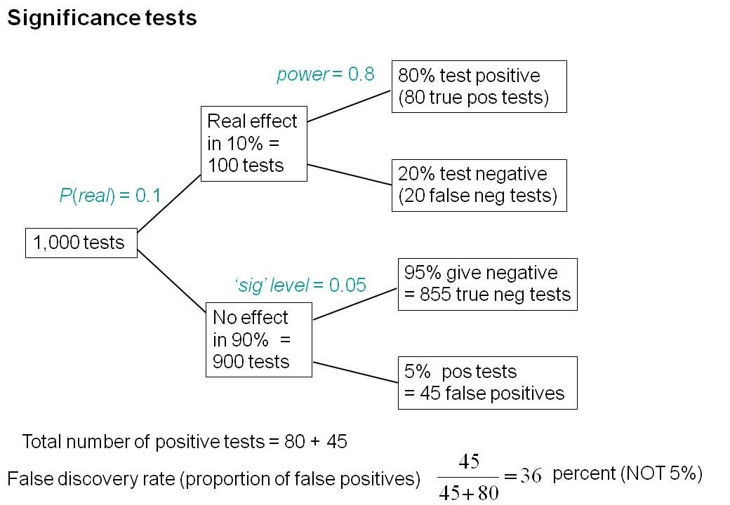
Suppose that we do 1000 tests. In 90% of them (900 tests) there is no real effect: the null hypothesis is true. If we use P = 0.05 as a criterion for significance then, according to the classical theory, 5% of them (45 tests) will give false positives, as shown in the lower limb of the tree diagram. If the power of the test was 0.8 then we’ll detect 80% of the real differences so there will be 80 correct positive tests.
The total number of positive tests is 45 + 80 = 125, and the proportion of these that are false positives is 45/125 = 36 percent. Our false discovery rate is far bigger than the 5% that many people still believe they are attaining.
In contrast, 98% of negative tests are right (though this is less surprising because 90% of experiments really have no effect).
The equation
You can skip this section without losing much.
As in the case of screening tests, this result can be calculated from an equation. The same equation works if we substitute power for sensitivity, P(real) for prevalence, and siglev for (1 – specificity) where siglev is the cut off value for “significance”, 0.05 in our examples.
The false discovery rate (the probability that, if a “signifcant” result is found, there is actually no real effect) is given by
\[FDR = \frac{siglev\left(1-P(real)\right)}{power.P(real) + siglev\left(1-P(real)\right) }\; \]
In the example above, power = 0.8, siglev = 0.05 and P(real) = 0.1, so the false discovery rate is
\[\frac{0.05 (1-0.1)}{0.8 \times 0.1 + 0.05 (1-0.1) }\; = 0.36 \]
So 36% of “significant” results are wrong, as found in the tree diagram.
Some subtleties
The argument just presented should be quite enough to convince you that significance testing, as commonly practised, will lead to disastrous numbers of false positives. But the basis of how to make inferences is still a matter that’s the subject of intense controversy among statisticians, so what is an experimenter to do?
It is difficult to give a consensus of informed opinion because, although there is much informed opinion, there is rather little consensus. A personal view follows. Colquhoun (1970), Lectures on Biostatistics, pp 94-95.
This is almost as true now as it was when I wrote it in the late 1960s, but there are some areas of broad agreement.
There are two subtleties that cause the approach outlined above to be a bit contentious. The first lies in the problem of deciding the prevalence, P(real). You may have noticed that if the frequency of real effects were 50% rather than 10%, the approach shown in the diagram would give a false discovery rate of only 6%, little different from the 5% that’s embedded in the consciousness of most experimentalists.
But this doesn’t get us off the hook, for two reasons. For a start, there is no reason at all to think that there will be a real effect there in half of the tests that we do. Of course if P(real) were even bigger than 0.5, the false discovery rate would fall to zero, because when P(real) = 1, all effects are real and therefore all positive tests are correct.
There is also a more subtle point. If we are trying to interpret the result of a single test that comes out with a P value of, say, P = 0.047, then we should not be looking at all significant results (those with P < 0.05), but only at those tests that come out with P = 0.047. This can be done quite easily by simulating a long series of t tests, and then restricting attention to those that come out with P values between, say, 0.045 and 0.05. When this is done we find that the false discovery rate is at least 26%. That’s for the best possible case where the sample size is good (power of the test is 0.8) and the prevalence of real effects is 0.5. When, as in the tree diagram, the prevalence of real effects is 0.1, the false discovery rate is 76%. That’s enough to justify Ioannidis’ statement that most published results are wrong.
One problem with all of the approaches mentioned above was the need to guess at the prevalence of real effects (that’s what a Bayesian would call the prior probability). James Berger and colleagues (Sellke et al., 2001) have proposed a way round this problem by looking at all possible prior distributions and so coming up with a minimum false discovery rate that holds universally. The conclusions are much the same as before. If you claim to have found an effects whenever you observe a P value just less than 0.05, you will come to the wrong conclusion in at least 29% of the tests that you do. If, on the other hand, you use P = 0.001, you’ll be wrong in only 1.8% of cases. Valen Johnson (2013) has reached similar conclusions by a related argument.
A three-sigma rule
As an alternative to insisting on P < 0.001 before claiming you’ve discovered something, you could use a 3-sigma rule. In other words, insist that an effect is at least three standard deviations away from the control value (as opposed to the two standard deviations that correspond to P = 0.05).
The three sigma rule means using P= 0.0027 as your cut off. This, according to Berger’s rule, implies a false discovery rate of (at least) 4.5%, not far from the value that many people mistakenly think is achieved by using P = 0.05 as a criterion.
Particle physicists go a lot further than this. They use a 5-sigma rule before announcing a new discovery. That corresponds to a P value of less than one in a million (0.57 x 10⁻⁶). According to Berger’s rule this corresponds to a false discovery rate of (at least) around 20 per million. Of course their experiments can’t be randomised usually, so it’s as well to be on the safe side.
Underpowered experiments
All of the problems discussed so far concern the near-ideal case. They assume that your sample size is big enough (power about 0.8 say) and that all of the assumptions made in the test are true, that there is no bias or cheating and that no negative results are suppressed. The real-life problems can only be worse. One way in which it is often worse is that sample sizes are too small, so the statistical power of the tests is low.
The problem of underpowered experiments has been known since 1962, but it has been ignored. Recently it has come back into prominence, thanks in large part to John Ioannidis and the crisis of reproducibility in some areas of science. Button et al. (2013) said
“We optimistically estimate the median statistical power of studies in the neuroscience field to be between about 8% and about 31%”
This is disastrously low. Running simulated t tests shows that with a power of 0.2, not only do you have only a 20% chance of detecting a real effect, but that when you do manage to get a “significant” result there is a 76% chance that it’s a false discovery.
And furthermore, when you do find a “significant” result, the size of the effect will be over-estimated by a factor of nearly 2. This “inflation effect” happens because only those experiments that happen, by chance, to have a larger-than-average effect size will be deemed to be “significant”.
What should you do to prevent making a fool of yourself?
The simulated t test results, and some other subtleties, will be described in a paper, and/or in a future post. But I hope that enough has been said here to convince you that there are real problems in the sort of statistical tests that are universal in the literature.
The blame for the crisis in reproducibility has several sources.
One of them is the self-imposed publish-or-perish culture, which values quantity over quality, and which has done enormous harm to science.
The mis-assessment of individuals by silly bibliometric methods has contributed to this harm. Of all the proposed methods, altmetrics is demonstrably the most idiotic. Yet some vice-chancellors have failed to understand that.
Another is scientists’ own vanity, which leads to the PR department issuing disgracefully hyped up press releases.
In some cases, the abstract of a paper states that a discovery has been made when the data say the opposite. This sort of spin is common in the quack world. Yet referees and editors get taken in by the ruse (e.g see this study of acupuncture).
The reluctance of many journals (and many authors) to publish negative results biases the whole literature in favour of positive results. This is so disastrous in clinical work that a pressure group has been started; altrials.net “All Trials Registered | All Results Reported”.
Yet another problem is that it has become very hard to get grants without putting your name on publications to which you have made little contribution. This leads to exploitation of young scientists by older ones (who fail to set a good example). Peter Lawrence has set out the problems.
And, most pertinent to this post, a widespread failure to understand properly what a significance test means must contribute to the problem. Young scientists are under such intense pressure to publish, they have no time to learn about statistics.
Here are some things that can be done.
- Notice that all statistical tests of significance assume that the treatments have been allocated at random. This means that application of significance tests to observational data, e.g. epidemiological surveys of diet and health, is not valid. You can’t expect to get the right answer. The easiest way to understand this assumption is to think about randomisation tests (which should have replaced t tests decades ago, but which are still rare). There is a simple introduction in Lectures on Biostatistics (chapters 8 and 9). There are other assumptions too, about the distribution of observations, independence of measurements), but randomisation is the most important.
- Never, ever, use the word “significant” in a paper. It is arbitrary, and, as we have seen, deeply misleading. Still less should you use “almost significant”, “tendency to significant” or any of the hundreds of similar circumlocutions listed by Matthew Hankins on his Still not Significant blog.
- If you do a significance test, just state the P value and give the effect size and confidence intervals (but be aware that this is just another way of expressing the P value approach: it tells you nothing whatsoever about the false discovery rate).
- Observation of a P value close to 0.05 means nothing more than ‘worth another look’. In practice, one’s attitude will depend on weighing the losses that ensue if you miss a real effect against the loss to your reputation if you claim falsely to have made a discovery.
- If you want to avoid making a fool of yourself most of the time, don’t regard anything bigger than P < 0.001 as a demonstration that you’ve discovered something. Or, slightly less stringently, use a three-sigma rule.
Despite the gigantic contributions that Ronald Fisher made to statistics, his work has been widely misinterpreted. We must, however reluctantly, concede that there is some truth in the comment made by an astute journalist:
“The plain fact is that 70 years ago Ronald Fisher gave scientists a mathematical machine for turning baloney into breakthroughs, and °flukes into funding. It is time to pull the plug“. Robert Matthews Sunday Telegraph, 13 September 1998.
There is now a video on YouTube that attempts to explain explain simply the essential ideas. The video has now been updated. The new version has better volume and it used term ‘false positive risk’, rather than the earlier term ‘false discovery rate’, to avoid confusion with the use of the latter term in the context of multiple comparisons.
The false positive risk: a proposal concerning what to do about p-values (version 2)
Follow-up
31 March 2014 I liked Stephen Senn’s first comment on twitter (the twitter stream is storified here). He said ” I may have to write a paper ‘You may believe you are NOT a Bayesian but you’re wrong'”. I maintain that the analysis here is merely an exercise in conditional probabilities. It bears a formal similarity to a Bayesian argument, but is free of more contentious parts of the Bayesian approach. This is amplified in a comment, below.
4 April 2014
I just noticed that my first boss, Heinz Otto Schild.in his 1942 paper about the statistical analysis of 2+2 dose biological assays (written while he was interned at the beginning of the war) chose to use 99% confidence limits, rather than the now universal 95% limits. The later are more flattering to your results, but Schild was more concerned with precision than self-promotion.
This post is about why screening healthy people is generally a bad idea. It is the first in a series of posts on the hazards of statistics.
There is nothing new about it: Graeme Archer recently wrote a similar piece in his Telegraph blog. But the problems are consistently ignored by people who suggest screening tests, and by journals that promote their work. It seems that it can’t be said often enough.
The reason is that most screening tests give a large number of false positives. If your test comes out positive, your chance of actually having the disease is almost always quite small. False positive tests cause alarm, and they may do real harm, when they lead to unnecessary surgery or other treatments.
Tests for Alzheimer’s disease have been in the news a lot recently. They make a good example, if only because it’s hard to see what good comes of being told early on that you might get Alzheimer’s later when there are no good treatments that can help with that news. But worse still, the news you are given is usually wrong anyway.
Consider a recent paper that described a test for "mild cognitive impairment" (MCI), a condition that may, but often isn’t, a precursor of Alzheimer’s disease. The 15-minute test was published in the Journal of Neuropsychiatry and Clinical Neurosciences by Scharre et al (2014). The test sounded pretty good. It had a specificity of 95% and a sensitivity of 80%.
Specificity (95%) means that 95% of people who are healthy will get the correct diagnosis: the test will be negative.
Sensitivity (80%) means that 80% of people who have MCI will get the correct diagnosis: the test will be positive.
To understand the implication of these numbers we need to know also the prevalence of MCI in the population that’s being tested. That was estimated as 1% of people have MCI. Or, for over-60s only, 5% of people have MCI. Now the calculation is easy. Suppose 10.000 people are tested. 1% (100 people) will have MCI, of which 80% (80 people) will be diagnosed correctly. And 9,900 do not have MCI, of which 95% will test negative (correctly). The numbers can be laid out in a tree diagram.
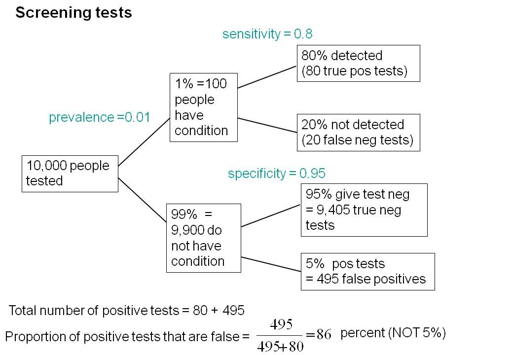
The total number of positive tests is 80 + 495 = 575, of which 495 are false positives. The fraction of tests that are false positives is 495/575= 86%.
Thus there is a 14% chance that if you test positive, you actually have MCI. 86% of people will be alarmed unnecessarily.
Even for people over 60. among whom 5% of the population have MC!, the test is gives the wrong result (54%) more often than it gives the right result (46%).
The test is clearly worse than useless. That was not made clear by the authors, or by the journal. It was not even made clear by NHS Choices.
It should have been.
It’s easy to put the tree diagram in the form of an equation. Denote sensitivity as sens, specificity as spec and prevalence as prev.
The probability that a positive test means that you actually have the condition is given by
\[\frac{sens.prev}{sens.prev + \left(1-spec\right)\left(1-prev\right) }\; \]
In the example above, sens = 0.8, spec = 0.95 and prev = 0.01, so the fraction of positive tests that give the right result is
\[\frac{0.8 \times 0.01}{0.8 \times 0.01 + \left(1 – 0.95 \right)\left(1 – 0.01\right) }\; = 0.139 \]
So 13.9% of positive tests are right, and 86% are wrong, as found in the tree diagram.
The lipid test for Alzheimers’
Another Alzheimers’ test has been in the headlines very recently. It performs even worse than the 15-minute test, but nobody seems to have noticed. It was published in Nature Medicine, by Mapstone et al. (2014). According to the paper, the sensitivity is 90% and the specificity is 90%, so, by constructing a tree, or by using the equation, the probability that you are ill, given that you test positive is a mere 8% (for a prevalence of 1%). And even for over-60s (prevalence 5%), the value is only 32%, so two-thirds of positive tests are still wrong. Again this was not pointed out by the authors. Nor was it mentioned by Nature Medicine in its commentary on the paper. And once again, NHS Choices missed the point.
Why does there seem to be a conspiracy of silence about the deficiencies of screening tests? It has been explained very clearly by people like Margaret McCartney who understand the problems very well. Is it that people are incapable of doing the calculations? Surely not. Is it that it’s better for funding to pretend you’ve invented a good test, when you haven’t? Do journals know that anything to do with Alzheimers’ will get into the headlines, and don’t want to pour cold water on a good story?
Whatever the explanation, it’s bad science that can harm people.
Follow-up
March 12 2014. This post was quickly picked up by the ampp3d blog, run by the Daily Mirror. Conrad Quilty-Harper showed some nice animations under the heading How a “90% accurate” Alzheimer’s test can be wrong 92% of the time.
March 12 2014.
As so often, the journal promoted the paper in a way that wasn’t totally accurate. Hype is more important than accuracy, I guess.
June 12 2014.
The empirical evidence shows that “general health checks” (a euphemism for mass screening of the healthy) simply don’t help. See review by Gøtzsche, Jørgensen & Krogsbøll (2014) in BMJ. They conclude
“Doctors should not offer general health checks to their patients,and governments should abstain from introducing health check programmes, as the Danish minister of health did when she learnt about the results of the Cochrane review and the Inter99 trial. Current programmes, like the one in the United Kingdom,should be abandoned.”
8 July 2014
Yet another over-hyped screening test for Alzheimer’s in the media. And once again. the hype originated in the press release, from Kings College London this time. The press release says
"They identified a combination of 10 proteins capable of predicting whether individuals with MCI would develop Alzheimer’s disease within a year, with an accuracy of 87 percent"
The term “accuracy” is not defined in the press release. And it isn’t defined in the original paper either. I’ve written to senior author, Simon Lovestone to try to find out what it means. The original paper says
"Sixteen proteins correlated with disease severity and cognitive decline. Strongest associations were in the MCI group with a panel of 10 proteins predicting progression to AD (accuracy 87%, sensitivity 85% and specificity 88%)."
A simple calculation, as shown above, tells us that with sensitivity 85% and specificity 88%. the fraction of people who have a positive test who are diagnosed correctly is 44%. So 56% of positive results are false alarms. These numbers assume that the prevalence of the condition in the population being tested is 10%, a higher value than assumed in other studies. If the prevalence were only 5% the results would be still worse: 73% of positive tests would be wrong. Either way, that’s not good enough to be useful as a diagnostic method.
In one of the other recent cases of Alzheimer’s tests, six months ago, NHS Choices fell into the same trap. They changed it a bit after I pointed out the problem in the comments. They seem to have learned their lesson because their post on this study was titled “Blood test for Alzheimer’s ‘no better than coin toss’ “. That’s based on the 56% of false alarms mention above.
The reports on BBC News and other media totally missed the point. But, as so often, their misleading reports were based on a misleading press release. That means that the university, and ultimately the authors, are to blame.
I do hope that the hype has no connection with the fact that Conflicts if Interest section of the paper says
"SL has patents filed jointly with Proteome Sciences plc related to these findings"
What it doesn’t mention is that, according to Google patents, Kings College London is also a patent holder, and so has a vested interest in promoting the product.
Is it really too much to expect that hard-pressed journalists might do a simple calculation, or phone someone who can do it for them? Until that happens, misleading reports will persist.
9 July 2014
It was disappointing to see that the usually excellent Sarah Boseley in the Guardian didn’t spot the problem either. And still more worrying that she quotes Dr James Pickett, head of research at the Alzheimer’s Society, as saying
These 10 proteins can predict conversion to dementia with less than 90% accuracy, meaning one in 10 people would get an incorrect result.
That number is quite wrong. It isn’t 1 in 10, it’s rather more than 1 in 2.
A resolution
After corresponding with the author, I now see what is going on more clearly.
The word "accuracy" was not defined in the paper, but was used in the press release and widely cited in the media. What it means is the ratio of the total number of true results (true positives + true negatives) to the total number of all results. This doesn’t seem to me to be useful number to give at all, because it conflates false negatives and false positives into a single number. If a condition is rare, the number of true negatives will be large (as shown above), but this does not make it a good test. What matters most to patients is not accuracy, defined in this way, but the false discovery rate.
The author makes it clear that the results are not intended to be a screening test for Alzheimer’s. It’s obvious from what’s been said that it would be a lousy test. Rather, the paper was intended to identify patients who would eventually (well, within only 18 months) get dementia. The denominator (always the key to statistical problems) in this case is the highly atypical patients that who come to memory clinics in trials centres (the potential trials population). The prevalence in this very restricted population may indeed be higher that the 10 percent that I used above.
Reading between the lines of the press release, you might have been able to infer some of thus (though not the meaning of “accuracy”). The fact that the media almost universally wrote up the story as a “breakthrough” in Alzeimer’s detection, is a consequence of the press release and of not reading the original paper.
I wonder whether it is proper for press releases to be issued at all for papers like this, which address a narrow technical question (selection of patients for trials). That us not a topic of great public interest. It’s asking for misinterpretation and that’s what it got.
I don’t suppose that it escaped the attention of the PR people at Kings that anything that refers to dementia is front page news, whether it’s of public interest or not. When we had an article in Nature in 2008, I remember long discussions about a press release with the arts graduate who wrote it (not at our request). In the end we decides that the topic was not of sufficient public interest to merit a press release and insisted that none was issued. Perhaps that’s what should have happened in this case too.
This discussion has certainly illustrated the value of post-publication peer review. See, especially, the perceptive comments, below, from Humphrey Rang and from Dr Aston and from Dr Kline.
14 July 2014. Sense about Science asked me to write a guest blog to explain more fully the meaning of "accuracy", as used in the paper and press release. It’s appeared on their site and will be reposted on this blog soon.