
Download Lectures on Biostatistics (1971). Corrected and searchable version of Google books edition
Download review of Lectures on Biostatistics (THES, 1973).
false positives
This piece is almost identical with today’s Spectator Health article.
This week there has been enormously wide coverage in the press for one of the worst papers on acupuncture that I’ve come across. As so often, the paper showed the opposite of what its title and press release, claimed. For another stunning example of this sleight of hand, try Acupuncturists show that acupuncture doesn’t work, but conclude the opposite: journal fails, published in the British Journal of General Practice).
Presumably the wide coverage was a result of the hyped-up press release issued by the journal, BMJ Acupuncture in Medicine. That is not the British Medical Journal of course, but it is, bafflingly, published by the BMJ Press group, and if you subscribe to press releases from the real BMJ. you also get them from Acupuncture in Medicine. The BMJ group should not be mixing up press releases about real medicine with press releases about quackery. There seems to be something about quackery that’s clickbait for the mainstream media.
As so often, the press release was shockingly misleading: It said
Acupuncture may alleviate babies’ excessive crying Needling twice weekly for 2 weeks reduced crying time significantly
This is totally untrue. Here’s why.
|
Luckily the Science Media Centre was on the case quickly: read their assessment. The paper made the most elementary of all statistical mistakes. It failed to make allowance for the jelly bean problem. The paper lists 24 different tests of statistical significance and focusses attention on three that happen to give a P value (just) less than 0.05, and so were declared to be "statistically significant". If you do enough tests, some are bound to come out “statistically significant” by chance. They are false postives, and the conclusions are as meaningless as “green jelly beans cause acne” in the cartoon. This is called P-hacking and it’s a well known cause of problems. It was evidently beyond the wit of the referees to notice this naive mistake. It’s very doubtful whether there is anything happening but random variability. And that’s before you even get to the problem of the weakness of the evidence provided by P values close to 0.05. There’s at least a 30% chance of such values being false positives, even if it were not for the jelly bean problem, and a lot more than 30% if the hypothesis being tested is implausible. I leave it to the reader to assess the plausibility of the hypothesis that a good way to stop a baby crying is to stick needles into the poor baby. If you want to know more about P values try Youtube or here, or here. |
|

One of the people asked for an opinion on the paper was George Lewith, the well-known apologist for all things quackish. He described the work as being a "good sized fastidious well conducted study ….. The outcome is clear". Thus showing an ignorance of statistics that would shame an undergraduate.
On the Today Programme, I was interviewed by the formidable John Humphrys, along with the mandatory member of the flat-earth society whom the BBC seems to feel obliged to invite along for "balance". In this case it was professional acupuncturist, Mike Cummings, who is an associate editor of the journal in which the paper appeared. Perhaps he’d read the Science media centre’s assessment before he came on, because he said, quite rightly, that
"in technical terms the study is negative" "the primary outcome did not turn out to be statistically significant"
to which Humphrys retorted, reasonably enough, “So it doesn’t work”. Cummings’ response to this was a lot of bluster about how unfair it was for NICE to expect a treatment to perform better than placebo. It was fascinating to hear Cummings admit that the press release by his own journal was simply wrong.
Listen to the interview here
Another obvious flaw of the study is that the nature of the control group. It is not stated very clearly but it seems that the baby was left alone with the acupuncturist for 10 minutes. A far better control would have been to have the baby cuddled by its mother, or by a nurse. That’s what was used by Olafsdottir et al (2001) in a study that showed cuddling worked just as well as another form of quackery, chiropractic, to stop babies crying.
Manufactured doubt is a potent weapon of the alternative medicine industry. It’s the same tactic as was used by the tobacco industry. You scrape together a few lousy papers like this one and use them to pretend that there’s a controversy. For years the tobacco industry used this tactic to try to persuade people that cigarettes didn’t give you cancer, and that nicotine wasn’t addictive. The main stream media obligingly invite the representatives of the industry who convey to the reader/listener that there is a controversy, when there isn’t.
Acupuncture is no longer controversial. It just doesn’t work -see Acupuncture is a theatrical placebo: the end of a myth. Try to imagine a pill that had been subjected to well over 3000 trials without anyone producing convincing evidence for a clinically useful effect. It would have been abandoned years ago. But by manufacturing doubt, the acupuncture industry has managed to keep its product in the news. Every paper on the subject ends with the words "more research is needed". No it isn’t.
Acupuncture is pre-scientific idea that was moribund everywhere, even in China, until it was revived by Mao Zedong as part of the appalling Great Proletarian Revolution. Now it is big business in China, and 100 percent of the clinical trials that come from China are positive.
if you believe them, you’ll truly believe anything.
Follow-up
29 January 2017
Soon after the Today programme in which we both appeared, the acupuncturist, Mike Cummings, posted his reaction to the programme. I thought it worth posting the original version in full. Its petulance and abusiveness are quite remarkable.
I thank Cummings for giving publicity to the video of our appearance, and for referring to my Wikipedia page. I leave it to the reader to judge my competence, and his, in the statistics of clinical trials. And it’s odd to be described as a "professional blogger" when the 400+ posts on dcscience.net don’t make a penny -in fact they cost me money. In contrast, he is the salaried medical director of the British Medical Acupuncture Society.
It’s very clear that he has no understanding of the error of the transposed conditional, nor even the mulltiple comparison problem (and neither, it seems, does he know the meaning of the word ‘protagonist’).
I ignored his piece, but several friends complained to the BMJ for allowing such abusive material on their blog site. As a result a few changes were made. The “baying mob” is still there, but the Wikipedia link has gone. I thought that readers might be interested to read the original unexpurgated version. It shows, better than I ever could, the weakness of the arguments of the alternative medicine community. To quote Upton Sinclair:
“It is difficult to get a man to understand something, when his salary depends upon his not understanding it.”
It also shows that the BBC still hasn’t learned the lessons in Steve Jones’ excellent “Review of impartiality and accuracy of the BBC’s coverage of science“. Every time I appear in such a programme, they feel obliged to invite a member of the flat earth society to propagate their make-believe.
Acupuncture for infantile colic – misdirection in the media or over-reaction from a sceptic blogger?26 Jan, 17 | by Dr Mike Cummings So there has been a big response to this paper press released by BMJ on behalf of the journal Acupuncture in Medicine. The response has been influenced by the usual characters – retired professors who are professional bloggers and vocal critics of anything in the realm of complementary medicine. They thrive on oiling up and flexing their EBM muscles for a baying mob of fellow sceptics (see my ‘stereotypical mental image’ here). Their target in this instant is a relatively small trial on acupuncture for infantile colic.[1] Deserving of being press released by virtue of being the largest to date in the field, but by no means because it gave a definitive answer to the question of the efficacy of acupuncture in the condition. We need to wait for an SR where the data from the 4 trials to date can be combined. So what about the research itself? I have already said that the trial was not definitive, but it was not a bad trial. It suffered from under-recruiting, which meant that it was underpowered in terms of the statistical analysis. But it was prospectively registered, had ethical approval and the protocol was published. Primary and secondary outcomes were clearly defined, and the only change from the published protocol was to combine the two acupuncture groups in an attempt to improve the statistical power because of under recruitment. The fact that this decision was made after the trial had begun means that the results would have to be considered speculative. For this reason the editors of Acupuncture in Medicine insisted on alteration of the language in which the conclusions were framed to reflect this level of uncertainty. DC has focussed on multiple statistical testing and p values. These are important considerations, and we could have insisted on more clarity in the paper. P values are a guide and the 0.05 level commonly adopted must be interpreted appropriately in the circumstances. In this paper there are no definitive conclusions, so the p values recorded are there to guide future hypothesis generation and trial design. There were over 50 p values reported in this paper, so by chance alone you must expect some to be below 0.05. If one is to claim statistical significance of an outcome at the 0.05 level, ie a 1:20 likelihood of the event happening by chance alone, you can only perform the test once. If you perform the test twice you must reduce the p value to 0.025 if you want to claim statistical significance of one or other of the tests. So now we must come to the predefined outcomes. They were clearly stated, and the results of these are the only ones relevant to the conclusions of the paper. The primary outcome was the relative reduction in total crying time (TC) at 2 weeks. There were two significance tests at this point for relative TC. For a statistically significant result, the p values would need to be less than or equal to 0.025 – neither was this low, hence my comment on the Radio 4 Today programme that this was technically a negative trial (more correctly ‘not a positive trial’ – it failed to disprove the null hypothesis ie that the samples were drawn from the same population and the acupuncture intervention did not change the population treated). Finally to the secondary outcome – this was the number of infants in each group who continued to fulfil the criteria for colic at the end of each intervention week. There were four tests of significance so we need to divide 0.05 by 4 to maintain the 1:20 chance of a random event ie only draw conclusions regarding statistical significance if any of the tests resulted in a p value at or below 0.0125. Two of the 4 tests were below this figure, so we say that the result is unlikely to have been chance alone in this case. With hindsight it might have been good to include this explanation in the paper itself, but as editors we must constantly balance how much we push authors to adjust their papers, and in this case the editor focussed on reducing the conclusions to being speculative rather than definitive. A significant result in a secondary outcome leads to a speculative conclusion that acupuncture ‘may’ be an effective treatment option… but further research will be needed etc… Now a final word on the 3000 plus acupuncture trials that DC loves to mention. His point is that there is no consistent evidence for acupuncture after over 3000 RCTs, so it clearly doesn’t work. He first quoted this figure in an editorial after discussing the largest, most statistically reliable meta-analysis to date – the Vickers et al IPDM.[2] DC admits that there is a small effect of acupuncture over sham, but follows the standard EBM mantra that it is too small to be clinically meaningful without ever considering the possibility that sham (gentle acupuncture plus context of acupuncture) can have clinically relevant effects when compared with conventional treatments. Perhaps now the best example of this is a network meta-analysis (NMA) using individual patient data (IPD), which clearly demonstrates benefits of sham acupuncture over usual care (a variety of best standard or usual care) in terms of health-related quality of life (HRQoL).[3] |
30 January 2017
I got an email from the BMJ asking me to take part in a BMJ Head-to-Head debate about acupuncture. I did one of these before, in 2007, but it generated more heat than light (the only good thing to come out of it was the joke about leprechauns). So here is my polite refusal.
|
Hello Thanks for the invitation, Perhaps you should read the piece that I wrote after the Today programme Why don’t you do these Head to Heads about genuine controversies? To do them about homeopathy or acupuncture is to fall for the “manufactured doubt” stratagem that was used so effectively by the tobacco industry to promote smoking. It’s the favourite tool of snake oil salesman too, and th BMJ should see that and not fall for their tricks. Such pieces night be good clickbait, but they are bad medicine and bad ethics. All the best David |
This post arose from a recent meeting at the Royal Society. It was organised by Julie Maxton to discuss the application of statistical methods to legal problems. I found myself sitting next to an Appeal Court Judge who wanted more explanation of the ideas. Here it is.
Some preliminaries
The papers that I wrote recently were about the problems associated with the interpretation of screening tests and tests of significance. They don’t allude to legal problems explicitly, though the problems are the same in principle. They are all open access. The first appeared in 2014:
http://rsos.royalsocietypublishing.org/content/1/3/140216
Since the first version of this post, March 2016, I’ve written two more papers and some popular pieces on the same topic. There’s a list of them at http://www.onemol.org.uk/?page_id=456.
I also made a video for YouTube of a recent talk.
In these papers I was interested in the false positive risk (also known as the false discovery rate) in tests of significance. It turned out to be alarmingly large. That has serious consequences for the credibility of the scientific literature. In legal terms, the false positive risk means the proportion of cases in which, on the basis of the evidence, a suspect is found guilty when in fact they are innocent. That has even more serious consequences.
Although most of what I want to say can be said without much algebra, it would perhaps be worth getting two things clear before we start.
The rules of probability.
(1) To get any understanding, it’s essential to understand the rules of probabilities, and, in particular, the idea of conditional probabilities. One source would be my old book, Lectures on Biostatistics (now free), The account on pages 19 to 24 give a pretty simple (I hope) description of what’s needed. Briefly, a vertical line is read as “given”, so Prob(evidence | not guilty) means the probability that the evidence would be observed given that the suspect was not guilty.
(2) Another potential confusion in this area is the relationship between odds and probability. The relationship between the probability of an event occurring, and the odds on the event can be illustrated by an example. If the probability of being right-handed is 0.9, then the probability of being not being right-handed is 0.1. That means that 9 people out of 10 are right-handed, and one person in 10 is not. In other words for every person who is not right-handed there are 9 who are right-handed. Thus the odds that a randomly-selected person is right-handed are 9 to 1. In symbols this can be written
\[ \mathrm{probability=\frac{odds}{1 + odds}} \]
In the example, the odds on being right-handed are 9 to 1, so the probability of being right-handed is 9 / (1+9) = 0.9.
Conversely,
\[ \mathrm{odds =\frac{probability}{1 – probability}} \]
In the example, the probability of being right-handed is 0.9, so the odds of being right-handed are 0.9 / (1 – 0.9) = 0.9 / 0.1 = 9 (to 1).
With these preliminaries out of the way, we can proceed to the problem.
The legal problem
The first problem lies in the fact that the answer depends on Bayes’ theorem. Although that was published in 1763, statisticians are still arguing about how it should be used to this day. In fact whenever it’s mentioned, statisticians tend to revert to internecine warfare, and forget about the user.
Bayes’ theorem can be stated in words as follows
\[ \mathrm{\text{posterior odds ratio} = \text{prior odds ratio} \times \text{likelihood ratio}} \]
“Posterior odds ratio” means the odds that the person is guilty, relative to the odds that they are innocent, in the light of the evidence, and that’s clearly what one wants to know. The “prior odds” are the odds that the person was guilty before any evidence was produced, and that is the really contentious bit.
Sometimes the need to specify the prior odds has been circumvented by using the likelihood ratio alone, but, as shown below, that isn’t a good solution.
The analogy with the use of screening tests to detect disease is illuminating.
Screening tests
A particularly straightforward application of Bayes’ theorem is in screening people to see whether or not they have a disease. It turns out, in many cases, that screening gives a lot more wrong results (false positives) than right ones. That’s especially true when the condition is rare (the prior odds that an individual suffers from the condition is small). The process of screening for disease has a lot in common with the screening of suspects for guilt. It matters because false positives in court are disastrous.
The screening problem is dealt with in sections 1 and 2 of my paper. or on this blog (and here). A bit of animation helps the slides, so you may prefer the Youtube version.
The rest of my paper applies similar ideas to tests of significance. In that case the prior probability is the probability that there is in fact a real effect, or, in the legal case, the probability that the suspect is guilty before any evidence has been presented. This is the slippery bit of the problem both conceptually, and because it’s hard to put a number on it.
But the examples below show that to ignore it, and to use the likelihood ratio alone, could result in many miscarriages of justice.
In the discussion of tests of significance, I took the view that it is not legitimate (in the absence of good data to the contrary) to assume any prior probability greater than 0.5. To do so would presume you know the answer before any evidence was presented. In the legal case a prior probability of 0.5 would mean assuming that there was a 50:50 chance that the suspect was guilty before any evidence was presented. A 50:50 probability of guilt before the evidence is known corresponds to a prior odds ratio of 1 (to 1) If that were true, the likelihood ratio would be a good way to represent the evidence, because the posterior odds ratio would be equal to the likelihood ratio.
It could be argued that 50:50 represents some sort of equipoise, but in the example below it is clearly too high, and if it is less that 50:50, use of the likelihood ratio runs a real risk of convicting an innocent person.
The following example is modified slightly from section 3 of a book chapter by Mortera and Dawid (2008). Philip Dawid is an eminent statistician who has written a lot about probability and the law, and he’s a member of the legal group of the Royal Statistical Society.
My version of the example removes most of the algebra, and uses different numbers.
Example: The island problem
The “island problem” (Eggleston 1983, Appendix 3) is an imaginary example that provides a good illustration of the uses and misuses of statistical logic in forensic identification.
A murder has been committed on an island, cut off from the outside world, on which 1001 (= N + 1) inhabitants remain. The forensic evidence at the scene consists of a measurement, x, on a “crime trace” characteristic, which can be assumed to come from the criminal. It might, for example, be a bit of the DNA sequence from the crime scene.
Say, for the sake of example, that the probability of a random member of the population having characteristic x is P = 0.004 (i.e. 0.4% ), so the probability that a random member of the population does not have the characteristic is 1 – P = 0.996. The mainland police arrive and arrest a random islander, Jack. It is found that Jack matches the crime trace. There is no other relevant evidence.
How should this match evidence be used to assess the claim that Jack is the murderer? We shall consider three arguments that have been used to address this question. The first is wrong. The second and third are right. (For illustration, we have taken N = 1000, P = 0.004.)
(1) Prosecutor’s fallacy
Prosecuting counsel, arguing according to his favourite fallacy, asserts that the probability that Jack is guilty is 1 – P , or 0.996, and that this proves guilt “beyond a reasonable doubt”.
The probability that Jack would show characteristic x if he were not guilty would be 0.4% i.e. Prob(Jack has x | not guilty) = 0.004. Therefore the probability of the evidence, given that Jack is guilty, Prob(Jack has x | Jack is guilty), is one 1 – 0.004 = 0.996.
But this is Prob(evidence | guilty) which is not what we want. What we need is the probability that Jack is guilty, given the evidence, P(Jack is guilty | Jack has characteristic x).
To mistake the latter for the former is the prosecutor’s fallacy, or the error of the transposed conditional.
Dawid gives an example that makes the distinction clear.
“As an analogy to help clarify and escape this common and seductive confusion, consider the difference between “the probability of having spots, if you have measles” -which is close to 1 and “the probability of having measles, if you have spots” -which, in the light of the many alternative possible explanations for spots, is much smaller.”
(2) Defence counter-argument
Counsel for the defence points out that, while the guilty party must have characteristic x, he isn’t the only person on the island to have this characteristic. Among the remaining N = 1000 innocent islanders, 0.4% have characteristic x, so the number who have it will be NP = 1000 x 0.004 = 4 . Hence the total number of islanders that have this characteristic must be 1 + NP = 5 . The match evidence means that Jack must be one of these 5 people, but does not otherwise distinguish him from any of the other members of it. Since just one of these is guilty, the probability that this is Jack is thus 1/5, or 0.2— very far from being “beyond all reasonable doubt”.
(3) Bayesian argument
The probability of the having characteristic x (the evidence) would be Prob(evidence | guilty) = 1 if Jack were guilty, but if Jack were not guilty it would be 0.4%, i.e. Prob(evidence | not guilty) = P. Hence the likelihood ratio in favour of guilt, on the basis of the evidence, is
\[ LR=\frac{\text{Prob(evidence } | \text{ guilty})}{\text{Prob(evidence }|\text{ not guilty})} = \frac{1}{P}=250 \]
In words, the evidence would be 250 times more probable if Jack were guilty than if he were innocent. While this seems strong evidence in favour of guilt, it still does not tell us what we want to know, namely the probability that Jack is guilty in the light of the evidence: Prob(guilty | evidence), or, equivalently, the odds ratio -the odds of guilt relative to odds of innocence, given the evidence,
To get that we must multiply the likelihood ratio by the prior odds on guilt, i.e. the odds on guilt before any evidence is presented. It’s often hard to get a numerical value for this. But in our artificial example, it is possible. We can argue that, in the absence of any other evidence, Jack is no more nor less likely to be the culprit than any other islander, so that the prior probability of guilt is 1/(N + 1), corresponding to prior odds on guilt of 1/N.
We can now apply Bayes’s theorem to obtain the posterior odds on guilt:
\[ \text {posterior odds} = \text{prior odds} \times LR = \left ( \frac{1}{N}\right ) \times \left ( \frac{1}{P} \right )= 0.25 \]
Thus the odds of guilt in the light of the evidence are 4 to 1 against. The corresponding posterior probability of guilt is
\[ Prob( \text{guilty } | \text{ evidence})= \frac{1}{1+NP}= \frac{1}{1+4}=0.2 \]
This is quite small –certainly no basis for a conviction.
This result is exactly the same as that given by the Defence Counter-argument’, (see above). That argument was simpler than the Bayesian argument. It didn’t explicitly use Bayes’ theorem, though it was implicit in the argument. The advantage of using the former is that it looks simpler. The advantage of the explicitly Bayesian argument is that it makes the assumptions more clear.
In summary The prosecutor’s fallacy suggested, quite wrongly, that the probability that Jack was guilty was 0.996. The likelihood ratio was 250, which also seems to suggest guilt, but it doesn’t give us the probability that we need. In stark contrast, the defence counsel’s argument, and equivalently, the Bayesian argument, suggested that the probability of Jack’s guilt as 0.2. or odds of 4 to 1 against guilt. The potential for wrong conviction is obvious.
Conclusions.
Although this argument uses an artificial example that is simpler than most real cases, it illustrates some important principles.
(1) The likelihood ratio is not a good way to evaluate evidence, unless there is good reason to believe that there is a 50:50 chance that the suspect is guilty before any evidence is presented.
(2) In order to calculate what we need, Prob(guilty | evidence), you need to give numerical values of how common the possession of characteristic x (the evidence) is the whole population of possible suspects (a reasonable value might be estimated in the case of DNA evidence), We also need to know the size of the population. In the case of the island example, this was 1000, but in general, that would be hard to answer and any answer might well be contested by an advocate who understood the problem.
These arguments lead to four conclusions.
(1) If a lawyer uses the prosecutor’s fallacy, (s)he should be told that it’s nonsense.
(2) If a lawyer advocates conviction on the basis of likelihood ratio alone, s(he) should be asked to justify the implicit assumption that there was a 50:50 chance that the suspect was guilty before any evidence was presented.
(3) If a lawyer uses Defence counter-argument, or, equivalently, the version of Bayesian argument given here, (s)he should be asked to justify the estimates of the numerical value given to the prevalence of x in the population (P) and the numerical value of the size of this population (N). A range of values of P and N could be used, to provide a range of possible values of the final result, the probability that the suspect is guilty in the light of the evidence.
(4) The example that was used is the simplest possible case. For more complex cases it would be advisable to ask a professional statistician. Some reliable people can be found at the Royal Statistical Society’s section on Statistics and the Law.
If you do ask a professional statistician, and they present you with a lot of mathematics, you should still ask these questions about precisely what assumptions were made, and ask for an estimate of the range of uncertainty in the value of Prob(guilty | evidence) which they produce.
Postscript: real cases
Another paper by Philip Dawid, Statistics and the Law, is interesting because it discusses some recent real cases: for example the wrongful conviction of Sally Clark because of the wrong calculation of the statistics for Sudden Infant Death Syndrome.
On Monday 21 March, 2016, Dr Waney Squier was struck off the medical register by the General Medical Council because they claimed that she misrepresented the evidence in cases of Shaken Baby Syndrome (SBS).
This verdict was questioned by many lawyers, including Michael Mansfield QC and Clive Stafford Smith, in a letter. “General Medical Council behaving like a modern inquisition”
The latter has already written “This shaken baby syndrome case is a dark day for science – and for justice“..
The evidence for SBS is based on the existence of a triad of signs (retinal bleeding, subdural bleeding and encephalopathy). It seems likely that these signs will be present if a baby has been shake, i.e Prob(triad | shaken) is high. But this is irrelevant to the question of guilt. For that we need Prob(shaken | triad). As far as I know, the data to calculate what matters are just not available.
It seem that the GMC may have fallen for the prosecutor’s fallacy. Or perhaps the establishment won’t tolerate arguments. One is reminded, once again, of the definition of clinical experience: “Making the same mistakes with increasing confidence over an impressive number of years.” (from A Sceptic’s Medical Dictionary by Michael O’Donnell. A Sceptic’s Medical Dictionary BMJ publishing, 1997).
Appendix (for nerds). Two forms of Bayes’ theorem
The form of Bayes’ theorem given at the start is expressed in terms of odds ratios. The same rule can be written in terms of probabilities. (This was the form used in the appendix of my paper.) For those interested in the details, it may help to define explicitly these two forms.
In terms of probabilities, the probability of guilt in the light of the evidence (what we want) is
\[ \text{Prob(guilty } | \text{ evidence}) = \text{Prob(evidence } | \text{ guilty}) \frac{\text{Prob(guilty })}{\text{Prob(evidence })} \]
In terms of odds ratios, the odds ratio on guilt, given the evidence (which is what we want) is
\[ \frac{ \text{Prob(guilty } | \text{ evidence})} {\text{Prob(not guilty } | \text{ evidence}} =
\left ( \frac{ \text{Prob(guilty)}} {\text {Prob((not guilty)}} \right )
\left ( \frac{ \text{Prob(evidence } | \text{ guilty})} {\text{Prob(evidence } | \text{ not guilty}} \right ) \]
or, in words,
\[ \text{posterior odds of guilt } =\text{prior odds of guilt} \times \text{likelihood ratio} \]
This is the precise form of the equation that was given in words at the beginning.
A derivation of the equivalence of these two forms is sketched in a document which you can download.
Follow-up
23 March 2016
It’s worth pointing out the following connection between the legal argument (above) and tests of significance.
(1) The likelihood ratio works only when there is a 50:50 chance that the suspect is guilty before any evidence is presented (so the prior probability of guilt is 0.5, or, equivalently, the prior odds ratio is 1).
(2) The false positive rate in signiifcance testing is close to the P value only when the prior probability of a real effect is 0.5, as shown in section 6 of the P value paper.
However there is another twist in the significance testing argument. The statement above is right if we take as a positive result any P < 0.05. If we want to interpret a value of P = 0.047 in a single test, then, as explained in section 10 of the P value paper, we should restrict attention to only those tests that give P close to 0.047. When that is done the false positive rate is 26% even when the prior is 0.5 (and much bigger than 30% if the prior is smaller –see extra Figure), That justifies the assertion that if you claim to have discovered something because you have observed P = 0.047 in a single test then there is a chance of at least 30% that you’ll be wrong. Is there, I wonder, any legal equivalent of this argument?
Chalkdust is a magazine published by students of maths from UCL Mathematics department. Judging by its first issue, it’s an excellent vehicle for popularisation of maths. I have a piece in the second issue
You can view the whole second issue on line, or download a pdf of the whole issue. Or a pdf of my bit only: On the Perils of P values.
The piece started out as another exposition of the interpretation of P values, but the whole of the first part turned into an explanation of the principles of randomisation tests. It beats me why anybody still does a Student’s t test. The idea of randomisation tests is very old. They are as powerful as t tests when the assumptions of the latter are fulfilled but a lot better when the assumptions are wrong (in the jargon, they are uniformly-most-powerful tests).
Not only that, but you need no mathematics to do a randomisation test, whereas you need a good deal of mathematics to follow Student’s 1908 paper. And the randomisation test makes transparently clear that random allocation of treatments is a basic and essential assumption that’s necessary for the the validity of any test of statistical significance.
I made a short video that explains the principles behind the randomisation tests, to go with the printed article (a bit of animation always helps).
When I first came across the principals of randomisation tests, i was entranced by the simplicity of the idea. Chapters 6 – 9 of my old textbook were written to popularise them. You can find much more detail there.
In fact it’s only towards the end that I reiterate the idea that P values don’t answer the question that experimenters want to ask, namely:- if I claim I have made a discovery because P is small, what’s the chance that I’ll be wrong?
If you want the full story on that, read my paper. The story it tells is not very original, but it still isn’t known to most experimenters (because most statisticians still don’t teach it on elementary courses). The paper must have struck a chord because it’s had over 80,000 full text views and more than 10,000 pdf downloads. It reached an altmetric score of 975 (since when it has been mysteriously declining). That’s gratifying, but it is also a condemnation of the use of metrics. The paper is not original and it’s quite simple, yet it’s had far more "impact" than anything to do with my real work.
If you want simpler versions than the full paper, try this blog (part 1 and part 2), or the Youtube video about misinterpretation of P values.
The R code for doing 2-sample randomisation tests
You can download a pdf file that describes the two R scripts. There are two different R programs.
One re-samples randomly a specified number of times (the default is 100,000 times, but you can do any number). Download two_sample_rantest.R
The other uses every possible sample -in the case of the two samples of 10 observations,it gives the distribution for all 184,756 ways of selecting 10 observations from 20. Download 2-sample-rantest-exact.R
The launch party
Today the people who organise Chalkdust magazine held a party in the mathematics department at UCL. The editorial director is a graduate student in maths, Rafael Prieto Curiel. He was, at one time in the Mexican police force (he said he’d suffered more crime in London than in Mexico City). He, and the rest of the team, are deeply impressive. They’ve done a terrific job. Support them.

The party cakes

Rafael Prieto doing the introduction

Rafael Prieto doing the introduction

Rafael Prieto and me

I got the T shirt
Decoding the T shirt
The top line is "I" because that’s the usual symbol for the square root of -1.
|
The second line is one of many equations that describe a heart shape. It can be plotted by calculating a matrix of values of the left hand side for a range of values of x and y. Then plot the contour for a values x and y for which the left hand side is equal to 1. Download R script for this. (Method suggested by Rafael Prieto Curiel.) |
 |
Follow-up
5 November 2015
The Mann-Whitney test
I was stimulated to write this follow-up because yesterday I was asked by a friend to comment on the fact that five different tests all gave identical P values, P = 0.0079. The paper in question was in Science magazine (see Fig. 1), so it wouldn’t surprise me if the statistics were done badly, but in this case there is an innocent explanation.
The Chalkdust article, and the video, are about randomisation tests done using the original observed numbers, so look at them before reading on. There is a more detailed explanation in Chapter 9 of Lectures on Biostatistics. Before it became feasible to do this sort of test, there was a simpler, and less efficient, version in which the observations were ranked in ascending order, and the observed values were replaced by their ranks. This was known as the Mann Whitney test. It had the virtue that because all the ‘observations’ were now integers, the number of possible results of resampling was limited so it was possible to construct tables to allow one to get a rough P value. Of course, replacing observations by their ranks throws away some information, and now that we have computers there is no need to use a Mann-Whitney test ever. But that’s what was used in this paper.
In the paper (Fig 1) comparisons are made between two groups (assumed to be independent) with 5 observations in each group. The 10 observations are just the ranks, 1, 2, 3, 4, 5, 6, 7, 8, 9, 10.
To do the randomisation test we select 5 of these numbers at random for sample A, and the other 5 are sample B. (Of course this supposes that the treatments were applied randomly in the real experiment, which is unlikely to be true.) In fact there are only 10!/(5!.5!) = 252 possible ways to select a sample of 5 from 10, so it’s easy to list all of them. In the case where there is no overlap between the groups, one group will contain the smallest observations (ranks 1, 2, 3, 4, 5, and the other group will contain the highest observations, ranks 6, 7, 8, 9, 10.
In this case, the sum of the ‘observations’ in group A is 15, and the sum for group B is 40.These add to the sum of the first 10 integers, 10.(10+1)/2 = 55. The mean (which corresponds to a difference between means of zero) is 55/2 = 27.5.
There are two ways of getting an allocation as extreme as this (first group low, as above, or second group low, the other tail of the distribution). The two tailed P value is therefore 2/252 = 0.0079. This will be the result whenever the two groups don’t overlap, regardless of the numerical values of the observations. It’s the smallest P value the test can produce with 5 observations in each group.
The whole randomisation distribution looks like this

In this case, the abscissa is the sum of the ranks in sample A, rather than the difference between means for the two groups (the latter is easily calculated from the former). The red line shows the observed value, 15. There is only one way to get a total of 15 for group A: it must contain the lowest 5 ranks (group A = 1, 2, 3, 4, 5). There is also only one way to get a total of 16 (group A = 1, 2, 3, 4, 6),and there are two ways of getting a total of 17 (group A = 1, 2, 3, 4, 7, or 1, 2, 3, 5, 6), But there are 20 different ways of getting a sum of 27 or 28 (which straddle the mean, 27.5). The printout (.txt file) from the R program that was used to generate the distribution is as follows.
|
Randomisation test: exact calculation all possible samples INPUTS: exact calculation: all possible samples OUTPUTS Result of t test
|
Some problems. Figure 1 alone shows 16 two-sample comparisons, but no correction for multiple comparisons seems to have been made. A crude Bonferroni correction would require replacement of a P = 0.05 threshold with P = 0.05/16 = 0.003. None of the 5 tests that gave P = 0.0079 reaches this level (of course the whole idea of a threshold level is absurd anyway).
Furthermore, even a single test that gave P = 0.0079 would be expected to have a false positive rate of around 10 percent
In the course of thinking about metrics, I keep coming across cases of over-promoted research. An early case was “Why honey isn’t a wonder cough cure: more academic spin“. More recently, I noticed these examples.
“Effect of Vitamin E and Memantine on Functional Decline in Alzheimer Disease".(Spoiler -very little), published in the Journal of the American Medical Association. ”
and ” Primary Prevention of Cardiovascular Disease with a Mediterranean Diet” , in the New England Journal of Medicine (which had second highest altmetric score in 2013)
and "Sleep Drives Metabolite Clearance from the Adult Brain", published in Science
In all these cases, misleading press releases were issued by the journals themselves and by the universities. These were copied out by hard-pressed journalists and made headlines that were certainly not merited by the work. In the last three cases, hyped up tweets came from the journals. The responsibility for this hype must eventually rest with the authors. The last two papers came second and fourth in the list of highest altmetric scores for 2013
Here are to two more very recent examples. It seems that every time I check a highly tweeted paper, it turns out that it is very second rate. Both papers involve fMRI imaging, and since the infamous dead salmon paper, I’ve been a bit sceptical about them. But that is irrelevant to what follows.
Boost your memory with electricity
That was a popular headline at the end of August. It referred to a paper in Science magazine:
“Targeted enhancement of cortical-hippocampal brain networks and associative memory” (Wang, JX et al, Science, 29 August, 2014)
This study was promoted by the Northwestern University "Electric current to brain boosts memory". And Science tweeted along the same lines.
|
Science‘s link did not lead to the paper, but rather to a puff piece, "Rebooting memory with magnets". Again all the emphasis was on memory, with the usual entirely speculative stuff about helping Alzheimer’s disease. But the paper itself was behind Science‘s paywall. You couldn’t read it unless your employer subscribed to Science.
|
 |
|
All the publicity led to much retweeting and a big altmetrics score. Given that the paper was not open access, it’s likely that most of the retweeters had not actually read the paper. |

|
When you read the paper, you found that is mostly not about memory at all. It was mostly about fMRI. In fact the only reference to memory was in a subsection of Figure 4. This is the evidence.
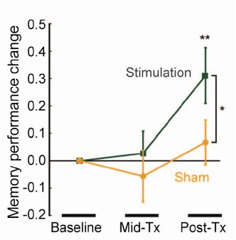
That looks desperately unconvincing to me. The test of significance gives P = 0.043. In an underpowered study like this, the chance of this being a false discovery is probably at least 50%. A result like this means, at most, "worth another look". It does not begin to justify all the hype that surrounded the paper. The journal, the university’s PR department, and ultimately the authors, must bear the responsibility for the unjustified claims.
Science does not allow online comments following the paper, but there are now plenty of sites that do. NHS Choices did a fairly good job of putting the paper into perspective, though they failed to notice the statistical weakness. A commenter on PubPeer noted that Science had recently announced that it would tighten statistical standards. In this case, they failed. The age of post-publication peer review is already reaching maturity
Boost your memory with cocoa
Another glamour journal, Nature Neuroscience, hit the headlines on October 26, 2014, in a paper that was publicised in a Nature podcast and a rather uninformative press release.
"Enhancing dentate gyrus function with dietary flavanols improves cognition in older adults. Brickman et al., Nat Neurosci. 2014. doi: 10.1038/nn.3850.".
The journal helpfully lists no fewer that 89 news items related to this study. Mostly they were something like “Drinking cocoa could improve your memory” (Kat Lay, in The Times). Only a handful of the 89 reports spotted the many problems.
A puff piece from Columbia University’s PR department quoted the senior author, Dr Small, making the dramatic claim that
“If a participant had the memory of a typical 60-year-old at the beginning of the study, after three months that person on average had the memory of a typical 30- or 40-year-old.”
|
Like anything to do with diet, the paper immediately got circulated on Twitter. No doubt most of the people who retweeted the message had not read the (paywalled) paper. The links almost all led to inaccurate press accounts, not to the paper itself. |
|

But some people actually read the paywalled paper and post-publication review soon kicked in. Pubmed Commons is a good site for that, because Pubmed is where a lot of people go for references. Hilda Bastian kicked off the comments there (her comment was picked out by Retraction Watch). Her conclusion was this.
"It’s good to see claims about dietary supplements tested. However, the results here rely on a chain of yet-to-be-validated assumptions that are still weakly supported at each point. In my opinion, the immodest title of this paper is not supported by its contents."
(Hilda Bastian runs the Statistically Funny blog -“The comedic possibilities of clinical epidemiology are known to be limitless”, and also a Scientific American blog about risk, Absolutely Maybe.)
NHS Choices spotted most of the problems too, in "A mug of cocoa is not a cure for memory problems". And so did Ian Musgrave of the University of Adelaide who wrote "Most Disappointing Headline Ever (No, Chocolate Will Not Improve Your Memory)",
Here are some of the many problems.
- The paper was not about cocoa. Drinks containing 900 mg cocoa flavanols (as much as in about 25 chocolate bars) and 138 mg of (−)-epicatechin were compared with much lower amounts of these compounds
- The abstract, all that most people could read, said that subjects were given "high or low cocoa–containing diet for 3 months". Bit it wasn’t a test of cocoa: it was a test of a dietary "supplement".
- The sample was small (37ppeople altogether, split between four groups), and therefore under-powered for detection of the small effect that was expected (and observed)
- The authors declared the result to be "significant" but you had to hunt through the paper to discover that this meant P = 0.04 (hint -it’s 6 lines above Table 1). That means that there is around a 50% chance that it’s a false discovery.
- The test was short -only three months
- The test didn’t measure memory anyway. It measured reaction speed, They did test memory retention too, and there was no detectable improvement. This was not mentioned in the abstract, Neither was the fact that exercise had no detectable effect.
- The study was funded by the Mars bar company. They, like many others, are clearly looking for a niche in the huge "supplement" market,
The claims by the senior author, in a Columbia promotional video that the drink produced "an improvement in memory" and "an improvement in memory performance by two or three decades" seem to have a very thin basis indeed. As has the statement that "we don’t need a pharmaceutical agent" to ameliorate a natural process (aging). High doses of supplements are pharmaceutical agents.
To be fair, the senior author did say, in the Columbia press release, that "the findings need to be replicated in a larger study—which he and his team plan to do". But there is no hint of this in the paper itself, or in the title of the press release "Dietary Flavanols Reverse Age-Related Memory Decline". The time for all the publicity is surely after a well-powered study, not before it.
The high altmetrics score for this paper is yet another blow to the reputation of altmetrics.
One may well ask why Nature Neuroscience and the Columbia press office allowed such extravagant claims to be made on such a flimsy basis.
What’s going wrong?
These two papers have much in common. Elaborate imaging studies are accompanied by poor functional tests. All the hype focusses on the latter. These led me to the speculation ( In Pubmed Commons) that what actually happens is as follows.
- Authors do big imaging (fMRI) study.
- Glamour journal says coloured blobs are no longer enough and refuses to publish without functional information.
- Authors tag on a small human study.
- Paper gets published.
- Hyped up press releases issued that refer mostly to the add on.
- Journal and authors are happy.
- But science is not advanced.
It’s no wonder that Dorothy Bishop wrote "High-impact journals: where newsworthiness trumps methodology".
It’s time we forgot glamour journals. Publish open access on the web with open comments. Post-publication peer review is working
But boycott commercial publishers who charge large amounts for open access. It shouldn’t cost more than about £200, and more and more are essentially free (my latest will appear shortly in Royal Society Open Science).
Follow-up
Hilda Bastian has an excellent post about the dangers of reading only the abstract "Science in the Abstract: Don’t Judge a Study by its Cover"
4 November 2014
I was upbraided on Twitter by Euan Adie, founder of Almetric.com, because I didn’t click through the altmetric symbol to look at the citations "shouldn’t have to tell you to look at the underlying data David" and "you could have saved a lot of Google time". But when I did do that, all I found was a list of media reports and blogs -pretty much the same as Nature Neuroscience provides itself.
More interesting, I found that my blog wasn’t listed and neither was PubMed Commons. When I asked why, I was told "needs to regularly cite primary research. PubMed, PMC or repository links”. But this paper is behind a paywall. So I provide (possibly illegally) a copy of it, so anyone can verify my comments. The result is that altmetric’s dumb algorithms ignore it. In order to get counted you have to provide links that lead nowhere.
So here’s a link to the abstract (only) in Pubmed for the Science paper http://www.ncbi.nlm.nih.gov/pubmed/25170153 and here’s the link for the Nature Neuroscience paper http://www.ncbi.nlm.nih.gov/pubmed/25344629
It seems that altmetrics doesn’t even do the job that it claims to do very efficiently.
It worked. By later in the day, this blog was listed in both Nature‘s metrics section and by altmetrics. com. But comments on Pubmed Commons were still missing, That’s bad because it’s an excellent place for post-publications peer review.
This post is about why screening healthy people is generally a bad idea. It is the first in a series of posts on the hazards of statistics.
There is nothing new about it: Graeme Archer recently wrote a similar piece in his Telegraph blog. But the problems are consistently ignored by people who suggest screening tests, and by journals that promote their work. It seems that it can’t be said often enough.
The reason is that most screening tests give a large number of false positives. If your test comes out positive, your chance of actually having the disease is almost always quite small. False positive tests cause alarm, and they may do real harm, when they lead to unnecessary surgery or other treatments.
Tests for Alzheimer’s disease have been in the news a lot recently. They make a good example, if only because it’s hard to see what good comes of being told early on that you might get Alzheimer’s later when there are no good treatments that can help with that news. But worse still, the news you are given is usually wrong anyway.
Consider a recent paper that described a test for "mild cognitive impairment" (MCI), a condition that may, but often isn’t, a precursor of Alzheimer’s disease. The 15-minute test was published in the Journal of Neuropsychiatry and Clinical Neurosciences by Scharre et al (2014). The test sounded pretty good. It had a specificity of 95% and a sensitivity of 80%.
Specificity (95%) means that 95% of people who are healthy will get the correct diagnosis: the test will be negative.
Sensitivity (80%) means that 80% of people who have MCI will get the correct diagnosis: the test will be positive.
To understand the implication of these numbers we need to know also the prevalence of MCI in the population that’s being tested. That was estimated as 1% of people have MCI. Or, for over-60s only, 5% of people have MCI. Now the calculation is easy. Suppose 10.000 people are tested. 1% (100 people) will have MCI, of which 80% (80 people) will be diagnosed correctly. And 9,900 do not have MCI, of which 95% will test negative (correctly). The numbers can be laid out in a tree diagram.
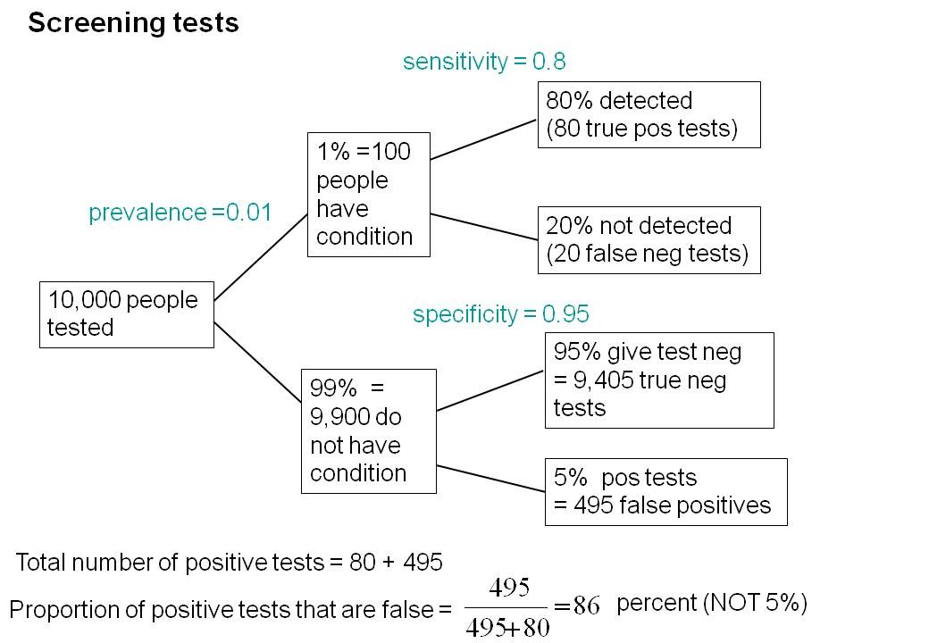
The total number of positive tests is 80 + 495 = 575, of which 495 are false positives. The fraction of tests that are false positives is 495/575= 86%.
Thus there is a 14% chance that if you test positive, you actually have MCI. 86% of people will be alarmed unnecessarily.
Even for people over 60. among whom 5% of the population have MC!, the test is gives the wrong result (54%) more often than it gives the right result (46%).
The test is clearly worse than useless. That was not made clear by the authors, or by the journal. It was not even made clear by NHS Choices.
It should have been.
It’s easy to put the tree diagram in the form of an equation. Denote sensitivity as sens, specificity as spec and prevalence as prev.
The probability that a positive test means that you actually have the condition is given by
\[\frac{sens.prev}{sens.prev + \left(1-spec\right)\left(1-prev\right) }\; \]
In the example above, sens = 0.8, spec = 0.95 and prev = 0.01, so the fraction of positive tests that give the right result is
\[\frac{0.8 \times 0.01}{0.8 \times 0.01 + \left(1 – 0.95 \right)\left(1 – 0.01\right) }\; = 0.139 \]
So 13.9% of positive tests are right, and 86% are wrong, as found in the tree diagram.
The lipid test for Alzheimers’
Another Alzheimers’ test has been in the headlines very recently. It performs even worse than the 15-minute test, but nobody seems to have noticed. It was published in Nature Medicine, by Mapstone et al. (2014). According to the paper, the sensitivity is 90% and the specificity is 90%, so, by constructing a tree, or by using the equation, the probability that you are ill, given that you test positive is a mere 8% (for a prevalence of 1%). And even for over-60s (prevalence 5%), the value is only 32%, so two-thirds of positive tests are still wrong. Again this was not pointed out by the authors. Nor was it mentioned by Nature Medicine in its commentary on the paper. And once again, NHS Choices missed the point.
Why does there seem to be a conspiracy of silence about the deficiencies of screening tests? It has been explained very clearly by people like Margaret McCartney who understand the problems very well. Is it that people are incapable of doing the calculations? Surely not. Is it that it’s better for funding to pretend you’ve invented a good test, when you haven’t? Do journals know that anything to do with Alzheimers’ will get into the headlines, and don’t want to pour cold water on a good story?
Whatever the explanation, it’s bad science that can harm people.
Follow-up
March 12 2014. This post was quickly picked up by the ampp3d blog, run by the Daily Mirror. Conrad Quilty-Harper showed some nice animations under the heading How a “90% accurate” Alzheimer’s test can be wrong 92% of the time.
March 12 2014.
As so often, the journal promoted the paper in a way that wasn’t totally accurate. Hype is more important than accuracy, I guess.
June 12 2014.
The empirical evidence shows that “general health checks” (a euphemism for mass screening of the healthy) simply don’t help. See review by Gøtzsche, Jørgensen & Krogsbøll (2014) in BMJ. They conclude
“Doctors should not offer general health checks to their patients,and governments should abstain from introducing health check programmes, as the Danish minister of health did when she learnt about the results of the Cochrane review and the Inter99 trial. Current programmes, like the one in the United Kingdom,should be abandoned.”
8 July 2014
Yet another over-hyped screening test for Alzheimer’s in the media. And once again. the hype originated in the press release, from Kings College London this time. The press release says
"They identified a combination of 10 proteins capable of predicting whether individuals with MCI would develop Alzheimer’s disease within a year, with an accuracy of 87 percent"
The term “accuracy” is not defined in the press release. And it isn’t defined in the original paper either. I’ve written to senior author, Simon Lovestone to try to find out what it means. The original paper says
"Sixteen proteins correlated with disease severity and cognitive decline. Strongest associations were in the MCI group with a panel of 10 proteins predicting progression to AD (accuracy 87%, sensitivity 85% and specificity 88%)."
A simple calculation, as shown above, tells us that with sensitivity 85% and specificity 88%. the fraction of people who have a positive test who are diagnosed correctly is 44%. So 56% of positive results are false alarms. These numbers assume that the prevalence of the condition in the population being tested is 10%, a higher value than assumed in other studies. If the prevalence were only 5% the results would be still worse: 73% of positive tests would be wrong. Either way, that’s not good enough to be useful as a diagnostic method.
In one of the other recent cases of Alzheimer’s tests, six months ago, NHS Choices fell into the same trap. They changed it a bit after I pointed out the problem in the comments. They seem to have learned their lesson because their post on this study was titled “Blood test for Alzheimer’s ‘no better than coin toss’ “. That’s based on the 56% of false alarms mention above.
The reports on BBC News and other media totally missed the point. But, as so often, their misleading reports were based on a misleading press release. That means that the university, and ultimately the authors, are to blame.
I do hope that the hype has no connection with the fact that Conflicts if Interest section of the paper says
"SL has patents filed jointly with Proteome Sciences plc related to these findings"
What it doesn’t mention is that, according to Google patents, Kings College London is also a patent holder, and so has a vested interest in promoting the product.
Is it really too much to expect that hard-pressed journalists might do a simple calculation, or phone someone who can do it for them? Until that happens, misleading reports will persist.
9 July 2014
It was disappointing to see that the usually excellent Sarah Boseley in the Guardian didn’t spot the problem either. And still more worrying that she quotes Dr James Pickett, head of research at the Alzheimer’s Society, as saying
These 10 proteins can predict conversion to dementia with less than 90% accuracy, meaning one in 10 people would get an incorrect result.
That number is quite wrong. It isn’t 1 in 10, it’s rather more than 1 in 2.
A resolution
After corresponding with the author, I now see what is going on more clearly.
The word "accuracy" was not defined in the paper, but was used in the press release and widely cited in the media. What it means is the ratio of the total number of true results (true positives + true negatives) to the total number of all results. This doesn’t seem to me to be useful number to give at all, because it conflates false negatives and false positives into a single number. If a condition is rare, the number of true negatives will be large (as shown above), but this does not make it a good test. What matters most to patients is not accuracy, defined in this way, but the false discovery rate.
The author makes it clear that the results are not intended to be a screening test for Alzheimer’s. It’s obvious from what’s been said that it would be a lousy test. Rather, the paper was intended to identify patients who would eventually (well, within only 18 months) get dementia. The denominator (always the key to statistical problems) in this case is the highly atypical patients that who come to memory clinics in trials centres (the potential trials population). The prevalence in this very restricted population may indeed be higher that the 10 percent that I used above.
Reading between the lines of the press release, you might have been able to infer some of thus (though not the meaning of “accuracy”). The fact that the media almost universally wrote up the story as a “breakthrough” in Alzeimer’s detection, is a consequence of the press release and of not reading the original paper.
I wonder whether it is proper for press releases to be issued at all for papers like this, which address a narrow technical question (selection of patients for trials). That us not a topic of great public interest. It’s asking for misinterpretation and that’s what it got.
I don’t suppose that it escaped the attention of the PR people at Kings that anything that refers to dementia is front page news, whether it’s of public interest or not. When we had an article in Nature in 2008, I remember long discussions about a press release with the arts graduate who wrote it (not at our request). In the end we decides that the topic was not of sufficient public interest to merit a press release and insisted that none was issued. Perhaps that’s what should have happened in this case too.
This discussion has certainly illustrated the value of post-publication peer review. See, especially, the perceptive comments, below, from Humphrey Rang and from Dr Aston and from Dr Kline.
14 July 2014. Sense about Science asked me to write a guest blog to explain more fully the meaning of "accuracy", as used in the paper and press release. It’s appeared on their site and will be reposted on this blog soon.